What Is a Median Filter?
A median filter is a non-linear filter that sorts the values within a sliding window and outputs the median (middle value) of those sorted samples.
Unlike linear filters such as the EMA filter or moving average filter , the median filter is exceptionally effective at removing impulse noise (spike-like noise) while preserving signal edges.
Common Applications
- Impulse noise removal: Sensor glitches, bit-flip errors in digital transmission
- Image processing: Salt-and-pepper noise removal
- Medical signal processing: ECG artifact removal
- Financial data: Filtering of erroneous tick data in price series
Mathematical Definition
For a window of size \(2m+1\) (where \(m\) is the one-sided half-width), the output \(y[n]\) at time \(n\) is:
\[ y[n] = \text{median}\bigl(x[n-m],\, x[n-m+1],\, \dots,\, x[n],\, \dots,\, x[n+m]\bigr) \tag{1} \]The \(2m+1\) values are sorted, and the \((m+1)\) -th value (the middle one) is selected as the output.
Example (window size \(= 5\) , \(m = 2\) ):
Suppose a portion of the input is \([\ldots, 3, 4, \mathbf{100}, 4, 3, \ldots]\) where the bold value is a spike:
\[ \text{sort}(3, 4, 100, 4, 3) = (3, 3, \mathbf{4}, 4, 100) \Rightarrow y[n] = 4 \tag{2} \]The spike value \(100\) is completely eliminated, and the true signal value \(4\) is recovered.
The Median as a Robust Statistic: Theoretical Grounding via the Breakdown Point
Rather than asserting by fiat that the median filter resists impulse noise, we derive it rigorously from the concept of the breakdown point in robust statistics. The breakdown point was introduced by Hampel (1971) as a quantitative measure of robustness — a single number that captures how “hard to break” an estimator is under contamination.
Definition of the Breakdown Point
Consider a sample \(x_1, \dots, x_n\) in which \(k\) of the points are replaced by arbitrary values \(z_1, \dots, z_k\) , forming a “contaminated sample.” The breakdown point \(\varepsilon^*\) of an estimator \(T\) is the smallest fraction of contaminated points that suffices to drive \(T\) ’s output to infinity, no matter how the contaminating values are chosen.
\[ \varepsilon^*(T, n) = \frac{1}{n} \min\Bigl\{ k \ge 1 : \sup_{z_1, \dots, z_k} \bigl| T(x_1, \dots, x_{n-k}, z_1, \dots, z_k) \bigr| = \infty \Bigr\} \]The smaller this value, the more fragile the estimator — a small number of outliers is enough to make it collapse.
The Mean’s Breakdown Point: 0%
For the sample mean \(\bar{x} = \frac{1}{n}\sum_i x_i\) , keep \(n-1\) points unchanged and replace only one point with \(z\) :
\[ \bar{x}_{\text{contaminated}} = \frac{(n-1)\,\bar{x}_{\text{clean}} + z}{n} \]As \(z \to \infty\) , \(\bar{x}_{\text{contaminated}} \to \infty\) . In other words, changing just one data point to an arbitrary value is enough to make the mean diverge:
\[ \varepsilon^*(\text{mean}, n) = \frac{1}{n} \xrightarrow[n \to \infty]{} 0 \]The mean’s breakdown point is 0%. No matter how large the sample size, this fragility — that a single point can send it to infinity — never goes away.
The Median’s Breakdown Point: 50%
Sort an odd-sized sample of \(n = 2p+1\) points in ascending order; the median is the \((p+1)\) -th order statistic. Now replace \(k\) data points with an arbitrarily large value \(z \to \infty\) ; after sorting, these contaminated points necessarily occupy the top \(k\) ranks.
- If \(k \le p\) (a minority): the \(k\) contaminated points are pushed to the top \(k\) ranks, leaving the remaining \(n-k \ge p+1\) clean points to occupy the lower ranks. As long as no more than \(p\) points are contaminated, the median’s rank \(p+1\) always falls within the set of clean points (the \((p+1)\) -th value from the bottom is simply the maximum of the clean points). The median is therefore bounded within the range of the clean data.
- The instant \(k = p+1\) (a majority): the contaminated points now occupy the top \(p+1\) ranks, and the median’s rank \(p+1\) finally falls among the contaminated points. The median then diverges together with \(z \to \infty\) .
The median therefore collapses exactly when a majority of the data is contaminated:
\[ \varepsilon^*(\text{median}, n) = \frac{p+1}{n} \xrightarrow[n \to \infty]{} \frac{1}{2} \]The median’s breakdown point is 50% — no matter how extreme the outliers, the median cannot be broken as long as fewer than half the samples are contaminated.
Numerical Verification
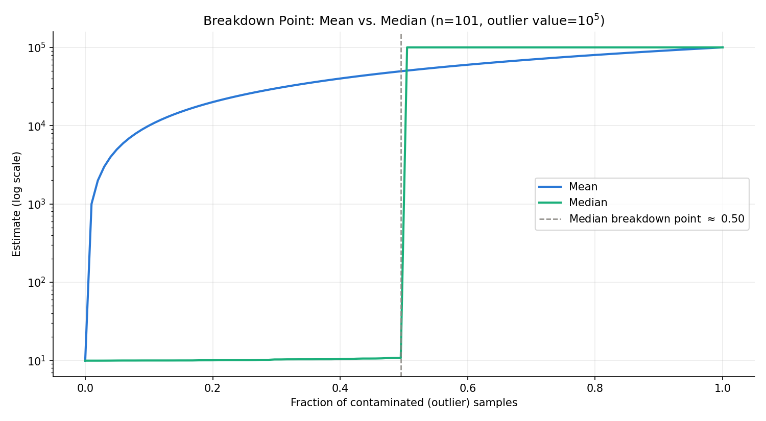
Starting from \(n=101\) clean data points (mean around 10), we replaced \(k\) of them with an outlier value (\(10^5\) ) and computed the mean and median as \(k\) ranges from \(0\) to \(101\) . The theoretical breakdown point is \(p/n = 50/101 \approx 0.495\) (below this fraction the median cannot collapse).
import numpy as np

n = 101
rng = np.random.default_rng(7)
base = 10 + 0.5 * rng.standard_normal(n)
outlier_value = 1e5

for k in [0, 50, 51, 101]:
    x = base.copy()
    x[:k] = outlier_value
    print(f"k={k:3d} (fraction={k/n:.3f}): mean={np.mean(x):.3e}, median={np.median(x):.3f}")
Results:
| \(k\) (contaminated) | Fraction | Mean | Median |
|---|---|---|---|
| 0 | 0.000 | \(9.91\) | \(9.94\) |
| 50 | 0.495 | \(4.95 \times 10^4\) | \(10.76\) (still within clean range) |
| 51 | 0.505 | \(5.05 \times 10^4\) | \(1.00 \times 10^5\) (broken down) |
| 101 | 1.000 | \(1.00 \times 10^5\) | \(1.00 \times 10^5\) |
Exactly as predicted, the median stays entirely within the clean range through \(k=50\) , then breaks down precisely at \(k=51\) (the majority threshold). The mean, in contrast, is already badly distorted by \(k=2\) — it moves from the clean value 10 to about 1990, a deviation of more than 190×. The figure below visualizes this result.
Direct Consequence for Impulse Noise Removal
If we view a windowed median filter as applying the “median estimator” locally to each window’s sample set, the breakdown-point theory above becomes a direct explanation of its impulse-noise robustness. For a window of size \(W=2m+1\) , let \(\rho\) denote the fraction of samples within the window that are corrupted by impulse noise:
- As long as \(\rho < 0.5\) (a majority of the window is clean), the output is theoretically guaranteed to lie within the range of the clean samples. Real-world impulse noise (given typical sensor false-detection rates or communication bit-error rates) is usually on the order of a few percent to the low tens of percent, so this condition is easily satisfied unless the window is pathologically narrow.
- Linear filters such as the moving average (a weighted sum), by contrast, have a breakdown point of \(1/W \to 0\) (a fragility that does not improve no matter how large the window is), so a single impulse anywhere in the window can severely distort the output.
This is the theoretical basis for why linear filters “spread” outliers to their neighbors while the median filter can “eliminate” them outright.
Key Differences from Linear Filters
The Superposition Principle Does Not Hold
Linear filters compute outputs as weighted sums of inputs. Median filtering involves sorting, so the superposition principle fails:
\[ \text{median}(ax_1 + bx_2) \neq a\cdot\text{median}(x_1) + b\cdot\text{median}(x_2) \tag{3} \]This non-linearity is precisely what gives the median filter its unique advantage over linear filters for impulse noise.
Impulse Noise Robustness
Linear filters spread impulse noise across neighboring samples. The median filter confines the spike’s influence within the window and eliminates it through sorting.
| Filter | Gaussian Noise Removal | Impulse Noise Removal | Edge Preservation |
|---|---|---|---|
| Moving Average | Good | Poor (spreads) | Low |
| EMA | Good (weighted) | Poor (spreads) | Low |
| Savitzky-Golay | Good | Poor | High |
| Median | Moderate | Excellent | High |
Python Implementation
Manual Implementation
import numpy as np

def median_filter_manual(x: np.ndarray, window_size: int) -> np.ndarray:
    """Median filter with reflect padding at edges."""
    assert window_size % 2 == 1, "window_size must be odd"
    m = window_size // 2
    n = len(x)
    y = np.empty(n)
    x_padded = np.pad(x, m, mode="reflect")
    for i in range(n):
        window = x_padded[i : i + window_size]
        y[i] = np.median(window)
    return y
Using scipy.signal.medfilt
In practice, scipy.signal.medfilt is the preferred choice:
import numpy as np
import matplotlib.pyplot as plt
from scipy import signal

# --- Signal generation ---
np.random.seed(42)
t = np.linspace(0, 1, 500)
x_clean = np.sin(2 * np.pi * 5 * t)
noise_gaussian = 0.2 * np.random.randn(len(t))
x_noisy = x_clean + noise_gaussian

# Add impulse noise
rng = np.random.default_rng(0)
impulse_indices = rng.choice(len(t), size=30, replace=False)
x_impulse = x_noisy.copy()
x_impulse[impulse_indices] += rng.choice([-4.0, 4.0], size=30)

# --- Apply filters ---
window_size = 11

y_median = signal.medfilt(x_impulse, kernel_size=window_size)
y_ma = np.convolve(x_impulse, np.ones(window_size) / window_size, mode="same")

# --- Plot ---
fig, axes = plt.subplots(3, 1, figsize=(12, 9), sharex=True)

axes[0].plot(t, x_impulse, color="gray", alpha=0.7, label="Noisy signal (with impulses)")
axes[0].plot(t, x_clean, color="blue", linestyle="--", label="Clean signal", linewidth=2)
axes[0].set_ylabel("Amplitude")
axes[0].legend()
axes[0].set_title("Input Signal (Impulse Noise Added)")

axes[1].plot(t, y_median, color="red", label=f"Median filter (window={window_size})")
axes[1].plot(t, x_clean, color="blue", linestyle="--", label="Clean signal", linewidth=2)
axes[1].set_ylabel("Amplitude")
axes[1].legend()
axes[1].set_title("Median Filter Output")

axes[2].plot(t, y_ma, color="green", label=f"Moving average (window={window_size})")
axes[2].plot(t, x_clean, color="blue", linestyle="--", label="Clean signal", linewidth=2)
axes[2].set_ylabel("Amplitude")
axes[2].set_xlabel("Time [s]")
axes[2].legend()
axes[2].set_title("Moving Average Output (Comparison)")

plt.tight_layout()
plt.show()
Quantitative Evaluation: PSNR Comparison of Impulse Noise Removal
The above was a visual comparison; let’s quantify the removal performance with an objective metric, PSNR (Peak Signal-to-Noise Ratio, in dB — higher means closer to the clean signal).
import numpy as np
from scipy import signal


def psnr(clean, test, data_range):
    mse = np.mean((clean - test) ** 2)
    if mse == 0:
        return np.inf
    return 10 * np.log10((data_range**2) / mse)


np.random.seed(42)
t = np.linspace(0, 1, 2000)
x_clean = np.sin(2 * np.pi * 5 * t)
data_range = x_clean.max() - x_clean.min()

window_size = 11
densities = [0.01, 0.02, 0.05, 0.1, 0.2, 0.3]  # impulse noise density

for density in densities:
    rng = np.random.default_rng(0)
    x_impulse = x_clean.copy()
    n_impulse = int(len(t) * density)
    idx = rng.choice(len(t), size=n_impulse, replace=False)
    x_impulse[idx] += rng.choice([-4.0, 4.0], size=n_impulse)

    y_median = signal.medfilt(x_impulse, kernel_size=window_size)
    y_ma = np.convolve(x_impulse, np.ones(window_size) / window_size, mode="same")

    print(
        f"density={density:.2f}: median={psnr(x_clean, y_median, data_range):.2f}dB, "
        f"moving_avg={psnr(x_clean, y_ma, data_range):.2f}dB"
    )
Results:
| Impulse noise density | Median filter PSNR | Moving-average PSNR | Gap |
|---|---|---|---|
| 1% | 57.22 dB | 24.39 dB | +32.8 dB |
| 2% | 54.30 dB | 21.44 dB | +32.9 dB |
| 5% | 49.68 dB | 17.21 dB | +32.5 dB |
| 10% | 46.54 dB | 14.09 dB | +32.5 dB |
| 20% | 43.30 dB | 11.33 dB | +32.0 dB |
| 30% | 16.29 dB | 9.47 dB | +6.8 dB |
Up to a density of 30%, the median filter maintains a roughly 30 dB PSNR advantage over the moving-average filter (more than a 30× amplitude-ratio improvement). At density 30%, however — even though this is still below the theoretical breakdown point for a window of 11 (majority threshold \(6/11 \approx 54.5\%\) ) — the median filter’s own PSNR drops sharply to 16.29 dB. This happens because, for window size 11 and contamination density 30%, the number of corrupted samples inside a given window follows \(\text{Binomial}(11, 0.3)\) , and the probability that this count reaches a majority (6 or more) rises to \(P(X \ge 6) \approx 7.8\%\) (compared to \(\approx 1.2\%\) at density 20% and \(\approx 0.03\%\) at density 10%). Even though the 50% breakdown point holds for any individual window, across many windows a non-negligible fraction happen to have a corrupted majority, dragging down the filter’s overall performance.
Window Size Selection
The window size \(W = 2m+1\) is the only parameter of the median filter.
import numpy as np
from scipy import signal
import matplotlib.pyplot as plt

np.random.seed(0)
t = np.linspace(0, 1, 300)
x_clean = np.sin(2 * np.pi * 3 * t)
x_noisy = x_clean.copy()
idx = np.random.choice(len(t), size=30, replace=False)
x_noisy[idx] += np.random.choice([-3, 3], size=30)

window_sizes = [3, 7, 15, 31]
fig, axes = plt.subplots(len(window_sizes), 1, figsize=(12, 10), sharex=True)

for ax, ws in zip(axes, window_sizes):
    y = signal.medfilt(x_noisy, kernel_size=ws)
    mse = np.mean((y - x_clean) ** 2)
    ax.plot(t, x_noisy, color="gray", alpha=0.5, label="Noisy input")
    ax.plot(t, y, color="red", label=f"window={ws}, MSE={mse:.4f}")
    ax.plot(t, x_clean, color="blue", linestyle="--", label="Clean signal", linewidth=1.5)
    ax.legend(loc="upper right")
    ax.set_ylabel("Amplitude")

axes[-1].set_xlabel("Time [s]")
plt.suptitle("Median Filter with Different Window Sizes")
plt.tight_layout()
plt.show()
Selection guidelines:
- Small window (3–5): Removes fine spikes while preserving signal detail. Suitable for sparse noise.
- Large window (11–31): Stronger denoising but may blunt sharp peaks and edges.
- Consecutive noise: The window size must exceed the length of any consecutive noise run.
Quantitative Evaluation: The Window-Size Trade-off Between Noise Removal and Edge Preservation
Increasing the window size improves noise removal, but how does it affect edge preservation? To find out, we superimposed Gaussian noise (\(\sigma=0.15\) ) and 20 impulse points onto a step signal (0 for the first half, 1 for the second half), and swept the window size from 3 to 199, measuring (1) noise-removal performance in the flat region (MSE) and (2) the edge transition width (the number of samples after the edge before the output settles within a tolerance of 0.1 of the target value).
import numpy as np
from scipy import signal

np.random.seed(3)
N = 400
x_step = np.concatenate([np.zeros(200), np.ones(200)])
rng3 = np.random.default_rng(4)
noise_flat = 0.15 * rng3.standard_normal(N)
impulse_idx = rng3.choice(N, size=20, replace=False)
x_step_noisy = x_step + noise_flat
x_step_noisy[impulse_idx] += rng3.choice([-2.0, 2.0], size=20)


def edge_transition_width(y, edge_pos=200, threshold=0.1, search=120):
    lo, hi = edge_pos - search, edge_pos + search
    seg = y[lo:hi]
    width = 0
    for i in range(len(seg)):
        pos = lo + i
        if pos < edge_pos:
            continue
        if abs(seg[i] - 1.0) > threshold:
            width += 1
        else:
            break
    return width


flat_region_idx = np.r_[20:180]
for ws in [3, 5, 7, 11, 15, 21, 31, 51, 71, 101, 151, 199]:
    y = signal.medfilt(x_step_noisy, kernel_size=ws)
    mse_flat = np.mean((y[flat_region_idx] - x_step[flat_region_idx]) ** 2)
    width = edge_transition_width(y, edge_pos=200, threshold=0.1)
    print(f"window={ws}: flat_MSE={mse_flat:.5f}, edge_width={width}")
Results:
| Window | Flat-region MSE | Edge transition width (samples) |
|---|---|---|
| 3 | 0.08887 | 5 |
| 5 | 0.00775 | 4 |
| 7 | 0.00500 | 3 |
| 11 | 0.00328 | 4 |
| 15 | 0.00240 | 4 |
| 21 | 0.00152 | 5 |
| 31 | 0.00079 | 5 |
| 51 | 0.00035 | 10 |
| 71 | 0.00030 | 12 |
| 101 | 0.00072 | 13 |
| 151 | 0.00152 | 21 |
| 199 | 0.00252 | 32 |
This result reveals a non-obvious finding. In the window range 3–31, flat-region noise removal improves monotonically (MSE drops about 110× from 0.089 to 0.0008), yet the edge transition width stays roughly constant (3–5 samples). This defies the intuition inherited from linear filters (that a larger window smooths edges more broadly): because the median filter selects an order statistic, the output remains step-shaped as long as one side of the edge still holds a majority within the window.
Beyond window 51, however, the improvement in flat-region MSE plateaus and then reverses (it bottoms out at 0.00030 at window 71, then worsens again at 101, 151, and 199), while the edge transition width expands sharply (10 at window 51, 32 at window 199). Once the window grows large enough to swallow up the edge itself or exceed the length of the flat region (200 samples in this example), the edge-preservation advantage begins to disappear. In practice, this quantitatively confirms a design guideline: keep the window size small relative to the scale of the structures you care about (flat-region length, edge spacing) — in this example, a window of 31 or smaller.
Adaptive Window-Width Design: The Adaptive Median Filter (AMF)
As the previous section showed, a fixed window size faces a dilemma: too small and it cannot remove strong noise; too large and it swallows structures wider than the window (edges, flat regions), destroying its own useful properties. The Adaptive Median Filter (AMF) mitigates this by dynamically varying the window size according to the signal’s local characteristics.
Design Philosophy
The classical adaptive median filter (Hwang & Haddad, 1995) applies a two-stage test to each sample of the signal:
- Is the window “informative”? Compute the minimum \(z_{\min}\) , maximum \(z_{\max}\) , and median \(z_{\text{med}}\) over the current window of size \(w\) , and check whether \(z_{\min} < z_{\text{med}} < z_{\max}\) . If this fails (likely meaning most of the window is corrupted by noise), grow the window to \(w \leftarrow w+2\) and re-test (once the cap \(w_{\max}\) is reached, output the median as-is).
- Is the center sample an outlier? If the above holds (the window is sufficiently informative), check whether the center sample \(x_c\) satisfies \(z_{\min} < x_c < z_{\max}\) . If it does, treat it as “not an outlier” and pass it through unchanged (i.e., no filtering); if not, treat it as an outlier and output the median \(z_{\text{med}}\) .
The key idea is that samples not flagged as noise are left completely untouched. Whereas a fixed-window median filter applies the median operation uniformly to every sample in the window, the AMF selectively corrects only the samples genuinely judged to be outliers, preserving as much of the signal’s true detail as possible.
Experimental Comparison: Fixed vs. Adaptive Window
We applied a simplified threshold-based adaptive median filter (window growing from 3 to 21; replace with the median whenever the deviation from it exceeds a threshold of 1.0, otherwise pass the center value through) to the same step signal used above (Gaussian noise + 20 impulse points), and compared it against a fixed window of 21.
import numpy as np
from scipy import signal

# --- Regenerate the same step signal (Gaussian noise + 20 impulse points) as before ---
np.random.seed(3)
N = 400
x_step = np.concatenate([np.zeros(200), np.ones(200)])
rng3 = np.random.default_rng(4)
noise_flat = 0.15 * rng3.standard_normal(N)
impulse_idx = rng3.choice(N, size=20, replace=False)
x_step_noisy = x_step + noise_flat
x_step_noisy[impulse_idx] += rng3.choice([-2.0, 2.0], size=20)
flat_region_idx = np.r_[20:180]


def adaptive_median_filter(x, w_min=3, w_max=21, impulse_thresh=1.0):
    n = len(x)
    half_max = w_max // 2
    x_padded = np.pad(x, half_max, mode="reflect")
    y = np.empty(n)
    for i in range(n):
        w = w_min
        while True:
            half = w // 2
            start = i + half_max - half
            window = x_padded[start : start + w]
            med = np.median(window)
            lo, hi = window.min(), window.max()
            center = x_padded[i + half_max]
            if (med - lo) > 0 and (hi - med) > 0:
                y[i] = med if abs(center - med) > impulse_thresh else center
                break
            w += 2
            if w > w_max:
                y[i] = med
                break
    return y


y_adaptive = adaptive_median_filter(x_step_noisy, w_min=3, w_max=21, impulse_thresh=1.0)
y_fixed21 = signal.medfilt(x_step_noisy, kernel_size=21)

impulse_in_flat = np.array([i for i in impulse_idx if i in flat_region_idx])
non_impulse_in_flat = np.array([i for i in flat_region_idx if i not in impulse_idx])

for name, y in [("raw (unfiltered)", x_step_noisy), ("fixed window=21", y_fixed21), ("adaptive (3..21)", y_adaptive)]:
    mse_impulse = np.mean((y[impulse_in_flat] - x_step[impulse_in_flat]) ** 2)
    mse_non_impulse = np.mean((y[non_impulse_in_flat] - x_step[non_impulse_in_flat]) ** 2)
    print(f"{name}: impulse_MSE={mse_impulse:.5f}, non_impulse_MSE={mse_non_impulse:.5f}")
Results (aggregated separately for the 8 impulse points and the non-impulse points within the flat region):
| Method | Impulse-location MSE | Non-impulse-location MSE |
|---|---|---|
| Raw observation (unfiltered) | 4.069 | 0.0213 |
| Fixed window=21 median | 0.00042 | 0.00158 |
| Adaptive median (3..21) | 1.264 | 0.0477 |
The fixed window (21) applies strong noise removal uniformly to every sample, nearly eliminating the impulse-location MSE (0.00042), but it keeps smoothing the non-impulse locations as well. The adaptive median filter, by contrast, reduces the impulse-location error to about a third of the raw value (4.069 → 1.264) while leaving non-impulse locations close to their raw values (0.0213 → 0.0477 — slightly worse near densely-clustered impulses, where the local median gets pulled a bit), passing through most of the signal’s genuine fluctuation untouched.
This result makes clear that the adaptive median filter is not simply an “all-around better filter” — it embodies a different design philosophy: selective correction versus uniform smoothing. Fixed, large-window filtering achieves better impulse-correction accuracy, but adaptive windowing better preserves detail in non-impulse regions.
Recent Research: Application to Scientific Instrumentation
The adaptive median filter remains an active area of improvement. In 2024, Guan et al. proposed an adaptive median filter called CODESmF in Scientific Reports, for removing salt-and-pepper noise from interference-fringe images captured by a Common-path Coherent-dispersion Spectrometer (CODES) used in exoplanet detection. The method consists of a noise-detection module based on submaximum/subminimum values and an adaptive median-filtering module that applies a variable window size (from \(3\times3\) to \(19\times19\) ) only to detected corrupted pixels, preserving the phase information essential to radial-velocity measurements while reducing phase/RV error caused by salt-and-pepper noise by more than 90% (about 98% in some conditions). This is a concrete example of the “selectively correct only the flagged corrupted points” design philosophy discussed in this section being actively researched at the frontier of precision instrumentation.
Deriving the Weighted Median Filter
An ordinary median filter treats every sample in the window equally, but the Weighted Median Filter (WMF) assigns a weight \(w_i \ge 0\) (an integer) to each position \(i\) , amplifying the “voice” of particular positions — typically the center.
Definition
For a window \(\{x_{n-m}, \dots, x_{n+m}\}\) with weights \(w_i\) , the weighted median is defined as the ordinary (equal-weight) median of the multiset formed by replicating each sample \(x_i\) exactly \(w_i\) times. Writing the total weight as \(W_{\text{tot}} = \sum_i w_i\) , the weighted median \(y\) is the value satisfying:
\[ \sum_{i:\, x_i < y} w_i < \frac{W_{\text{tot}}}{2} \quad \text{and} \quad \sum_{i:\, x_i \le y} w_i \ge \frac{W_{\text{tot}}}{2} \]When all \(w_i = 1\) , this reduces to the ordinary median filter.
Center Weight and Edge Preservation
Increasing only the center sample’s weight \(w_0\) (leaving the rest at \(w_i=1\) ) makes the center sample’s “votes” more dominant within the multiset. Applying the breakdown-point theory above to this multiset: the moment the center’s vote count exceeds the overall majority threshold \(W_{\text{tot}}/2\) , the weighted median always equals the center sample’s value regardless of the surrounding samples (i.e., the filter degenerates into the identity map). In other words, tuning the center weight acts as a continuous knob bridging from “an ordinary median” (\(w_0=1\) ) to “no filtering at all” (\(w_0\) at or above the majority threshold).
Experimental Verification
We applied the weighted median filter with center weight \(w_0 \in \{1, 3, 7, 15\}\) to the same step signal (noise + impulses) used above, using a half-width of 7 (window size 15).
import numpy as np

# --- Regenerate the same step signal (Gaussian noise + 20 impulse points) as before ---
np.random.seed(3)
N = 400
x_step = np.concatenate([np.zeros(200), np.ones(200)])
rng3 = np.random.default_rng(4)
noise_flat = 0.15 * rng3.standard_normal(N)
impulse_idx = rng3.choice(N, size=20, replace=False)
x_step_noisy = x_step + noise_flat
x_step_noisy[impulse_idx] += rng3.choice([-2.0, 2.0], size=20)
flat_region_idx = np.r_[20:180]


def edge_transition_width(y, edge_pos=200, threshold=0.1, search=120):
    lo, hi = edge_pos - search, edge_pos + search
    seg = y[lo:hi]
    width = 0
    for i in range(len(seg)):
        pos = lo + i
        if pos < edge_pos:
            continue
        if abs(seg[i] - 1.0) > threshold:
            width += 1
        else:
            break
    return width


def weighted_median_filter(x, half_width, center_weight):
    n = len(x)
    x_padded = np.pad(x, half_width, mode="reflect")
    y = np.empty(n)
    for i in range(n):
        window = list(x_padded[i : i + 2 * half_width + 1])
        center_val = x_padded[i + half_width]
        window += [center_val] * (center_weight - 1)
        y[i] = np.median(window)
    return y


for cw in [1, 3, 7, 15]:
    y_w = weighted_median_filter(x_step_noisy, half_width=7, center_weight=cw)
    mse_flat_w = np.mean((y_w[flat_region_idx] - x_step[flat_region_idx]) ** 2)
    width_w = edge_transition_width(y_w, edge_pos=200, threshold=0.1)
    print(f"center_weight={cw}: flat_MSE={mse_flat_w:.5f}, edge_width={width_w}")
Results:
| Center weight \(w_0\) | Flat-region MSE | Edge transition width |
|---|---|---|
| 1 (ordinary median) | 0.00240 | 4 |
| 3 | 0.00321 | 4 |
| 7 | 0.00696 | 1 |
| 15 | 0.22367 | 6 |
At \(w_0=7\) (window 15, total votes \(15+6=21\) , center holding 7 votes), the edge transition width improved dramatically from 4 samples to just 1, at the cost of flat-region MSE worsening by about 2.9×. A larger center weight makes the filter less likely to be “outvoted” by samples on the opposite side of an edge.
Pushing further to \(w_0=15\) (total votes \(15+14=29\) , center holding \(1+14=15\) votes — 51.7%, a majority) causes the output to degenerate almost entirely into the center sample itself (no filtering at all), exactly as the breakdown-point theory predicts, and flat-region MSE worsens to 0.224 (because impulses now pass straight through unfiltered). This is not a case of “more weight is always better” — it experimentally confirms that once the center weight exceeds the window’s majority threshold, the filter loses its meaning as a filter, an upper bound that follows directly from breakdown-point theory.
Relationship to the Bilateral Filter
Another well-known technique that, like the median filter, aims at “edge-preserving smoothing” is the Bilateral Filter (Tomasi & Manduchi, 1998). The two share a goal but achieve it through entirely different mathematical mechanisms.
The bilateral filter is a weighted linear combination using the product of a spatial weight (domain kernel) and an amplitude-difference weight (range kernel):
\[ y[n] = \frac{1}{W_n} \sum_{i \in \text{window}} x_i \cdot \exp\!\left(-\frac{(i-n)^2}{2\sigma_s^2}\right) \cdot \exp\!\left(-\frac{(x_i - x_n)^2}{2\sigma_r^2}\right) \](where \(W_n\) is the normalizing constant, \(\sigma_s\) controls the spread of the spatial kernel, and \(\sigma_r\) controls the spread of the range kernel). The median filter, in contrast, is a selection of an order statistic (Eq. (1)). The differences are summarized below.
| Aspect | Median filter | Bilateral filter |
|---|---|---|
| Type of operation | Order statistic (sort, select median) | Weighted linear combination (sum of value × kernel weight) |
| Mechanism of edge preservation | Majority-rule principle (50% breakdown) | Exponential decay of weight for “dissimilar” values via the range kernel |
| Robustness to a single extreme outlier | Bounded (rigorously guaranteed by breakdown-point theory) | Depends on \(\sigma_r\) . Its own weight decays exponentially as the difference grows, so it is practically robust, but there is no theoretical guarantee of boundedness |
| Number of parameters | 1 (window size \(W\) ) | 2 (\(\sigma_s\) , \(\sigma_r\) ) |
| Typical domain | Applies naturally to both 1D signals and images | Mainly images (2D); requires a notion of amplitude difference |
| Complexity | \(O(NW\log W)\) (fast algorithms exist) | Naively \(O(NW^2)\) ; fast approximations required |
Interestingly, the bilateral filter also has some practical resistance to impulse noise. As an outlier \(x_i\) moves further from the center value \(x_n\) , the range kernel \(\exp(-(x_i-x_n)^2/2\sigma_r^2)\) itself decays exponentially toward zero, so the outlier’s contribution to the weighted sum vanishes along with it. However, this is not the kind of guarantee the breakdown point provides — “bounded up to a specific fraction, no matter how extreme” — but rather a continuous, empirical robustness that depends on how \(\sigma_r\) is set (which in turn depends on prior knowledge of the noise amplitude). This is fundamentally different from the median filter’s discrete, combinatorial guarantee. The bilateral filter also performs well against low-amplitude Gaussian noise, but for spiky, large-amplitude impulse noise, the range kernel may fail to fully exclude its influence unless \(\sigma_r\) is set appropriately — which is why the median filter, specialized for impulse noise, remains the better choice in that regime.
Combining with EMA for Mixed Noise
The median filter excels at impulse noise but is only moderate for Gaussian noise. A practical two-stage pipeline combines both:
from scipy import signal
import numpy as np

def hybrid_filter(x: np.ndarray, median_window: int = 5, ema_alpha: float = 0.2) -> np.ndarray:
    """
    Two-stage filter: Median → EMA
    Step 1: Remove impulse noise with median filter
    Step 2: Smooth residual Gaussian noise with EMA
    """
    # Step 1: Impulse removal
    y_median = signal.medfilt(x, kernel_size=median_window)
    # Step 2: EMA smoothing
    y_ema = np.zeros_like(y_median)
    y_ema[0] = y_median[0]
    for i in range(1, len(y_median)):
        y_ema[i] = ema_alpha * y_median[i] + (1 - ema_alpha) * y_ema[i - 1]
    return y_ema
This two-stage design is widely used in sensor data pipelines and communication system denoising.
Computational Complexity and Edge Handling
Complexity
A naive implementation sorts \(W\)
values per output sample, giving \(O(W \log W)\)
per sample and \(O(NW \log W)\)
overall. scipy.signal.medfilt uses efficient internal algorithms. For large-scale data, scipy.ndimage.median_filter is often faster and offers more flexible edge-handling options:
from scipy import ndimage

# reflect padding (generally recommended)
y_reflect = ndimage.median_filter(x, size=11, mode="reflect")
# nearest-neighbor padding
y_nearest = ndimage.median_filter(x, size=11, mode="nearest")
Edge Handling (Overview)
scipy.signal.medfilt uses zero-padding by default. To control edge handling, use the mode parameter of scipy.ndimage.median_filter:
# reflect: mirror padding
y_reflect = ndimage.median_filter(x, size=11, mode="reflect")
# nearest: pad with the edge value
y_nearest = ndimage.median_filter(x, size=11, mode="nearest")
The right choice depends on the signal, as the next section examines in detail.
Edge Cases in Boundary Handling
When a median filter of window size \(W=2m+1\) is applied near the edges of a signal (\(n < m\) or \(n > N-1-m\) ), part of the window falls outside the signal’s domain. How this “overhang” is filled determines the output’s behavior near the boundary. We compare four common strategies.
| Strategy | Definition | Pros | Cons |
|---|---|---|---|
Zero-padding (the medfilt default) | Fill the out-of-range region with 0 | Simple to implement | Introduces an artificial discontinuity at the boundary if the signal is not near zero |
| Mirroring (reflect) | Fold the signal back across the boundary | Preserves continuity for smooth signals | Can over/under-estimate on a sloped region; risks duplicating a boundary-adjacent outlier |
| Edge replication (nearest) | Repeat the boundary value | Minimal boundary bias for monotone/quasi-static signals | Lags behind if the signal changes rapidly near the boundary |
| Truncation (valid-only output) | Output only where the window fits entirely within the signal | No bias is introduced in principle | The output is shorter than the input, requiring care downstream |
Experiment (1): Systematic Bias on a Clean Ramp Signal
First, we isolate the systematic bias inherent to each boundary strategy using a noise-free, monotonically increasing ramp signal (\(x[n]=n\) , \(n=0,\dots,199\) ).
import numpy as np
from scipy import signal, ndimage

N_ramp = 200
x_ramp = np.arange(N_ramp, dtype=float)
window3 = 15
m3 = window3 // 2

y_zero = signal.medfilt(x_ramp, kernel_size=window3)
y_reflect = ndimage.median_filter(x_ramp, size=window3, mode="reflect")
y_nearest = ndimage.median_filter(x_ramp, size=window3, mode="nearest")

boundary_idx = np.r_[0:m3, N_ramp - m3 : N_ramp]
for name, y in [("zero", y_zero), ("reflect", y_reflect), ("nearest", y_nearest)]:
    bias = np.mean(np.abs(y[boundary_idx] - x_ramp[boundary_idx]))
    print(f"{name}: mean |bias| at boundary = {bias:.3f}")
Results:
| Strategy | Mean absolute bias at boundary |
|---|---|
| Zero-padding | 2.000 |
| Mirroring (reflect) | 0.857 |
| Edge replication (nearest) | 0.000 |
For a monotone signal, edge replication (nearest) achieves exactly zero bias, as theory predicts: even when the window is filled with copies of the boundary value, the rank of the median position (\((m+1)\) -th) doesn’t change, because extending a monotone signal with replicated values preserves the ordering. Zero-padding, on the other hand, introduces a value (0) that is far from the signal’s true scale, which drags the median’s rank and produces a systematic bias (mean 2.0). Mirroring introduces values pointing in the opposite direction of the slope, which slightly over/under-estimates on a monotone incline (bias 0.857) — better than zero-padding, since at least the values are on the signal’s actual scale, but not perfect.
Experiment (2): An Impulse Near the Boundary
Next, in a more realistic scenario, we compare boundary-region and interior MSE for a noisy signal with impulses (sinusoid + 15 impulse points, \(N=200\) , window size 15).
import numpy as np
from scipy import signal, ndimage

np.random.seed(1)
t2 = np.linspace(0, 1, 200)
x_clean2 = np.sin(2 * np.pi * 3 * t2) + 0.3
rng2 = np.random.default_rng(2)
idx2 = rng2.choice(len(t2), size=15, replace=False)
x_noisy2 = x_clean2.copy()
x_noisy2[idx2] += rng2.choice([-3.0, 3.0], size=15)

window_size2 = 15
m2 = window_size2 // 2

y_zero = signal.medfilt(x_noisy2, kernel_size=window_size2)
y_reflect = ndimage.median_filter(x_noisy2, size=window_size2, mode="reflect")
y_nearest = ndimage.median_filter(x_noisy2, size=window_size2, mode="nearest")
y_constant = ndimage.median_filter(x_noisy2, size=window_size2, mode="constant")

boundary_idx = np.r_[0:m2, len(t2) - m2 : len(t2)]
interior_idx = np.r_[m2 : len(t2) - m2]
for name, y in [("zero", y_zero), ("reflect", y_reflect), ("nearest", y_nearest), ("constant", y_constant)]:
    mse_boundary = np.mean((y[boundary_idx] - x_clean2[boundary_idx]) ** 2)
    mse_interior = np.mean((y[interior_idx] - x_clean2[interior_idx]) ** 2)
    print(f"{name}: boundary_MSE={mse_boundary:.4f}, interior_MSE={mse_interior:.4f}")
Results:
| Strategy | Boundary-region MSE | Interior MSE |
|---|---|---|
| Zero-padding | 0.0123 | 0.0023 |
| Mirroring (reflect) | 0.0299 | 0.0023 |
| Edge replication (nearest) | 0.0020 | 0.0023 |
Constant-0 padding (ndimage, constant) | 0.0123 | 0.0023 |
In this experiment, mirroring performed worst. Investigating the cause: one of the randomly placed impulses sits just 4 samples from the right boundary (index 196, signal length 200, half-window 7), and mirroring folds this impulse into the virtual samples outside the boundary, duplicating it — so several output samples near the boundary end up affected by this one impulse more than they should. This is not a general rule that “mirroring is always worse”; rather, it is a concrete example of an edge case specific to mirroring: when an impulse sits near the boundary, mirroring risks making it appear in the window more often than it actually does. Edge replication (nearest) again benefited from its low systematic bias and produced the best result in this case as well.
Guidelines
- If the signal’s scale is far from zero, or the signal has a trend, avoid zero-padding (note that
scipy.signal.medfiltuses zero-padding by default). - For general-purpose data, edge replication (nearest) or mirroring (reflect) are both safe choices. However, since mirroring can be disadvantageous when impulses cluster near the boundary, edge replication is more predictable when the noise characteristics near the boundary are unknown.
- For applications where the boundary’s behavior itself affects the reliability of the result (e.g., evaluating endpoints of measurement data), consider truncation, discarding the inherently uncertain boundary output altogether.
Recent Research Trends: Positioning Classical Filters Against Deep-Learning Denoising
Here we situate the median filter, as a representative classical non-linear filter, relative to deep-learning-based denoising (e.g., DnCNN), based on literature from 2023 onward.
Elad, Kawar, and Vaksman’s 2023 survey “Image Denoising: The Deep Learning Revolution and Beyond” (arXiv:2301.03362) recalls that, roughly a decade before the survey’s publication, the research community widely believed that “denoising was a dead problem” — essentially solved, with little room for further gains. The rise of deep learning overturned this assumption, not only revolutionizing denoising performance itself but also greatly expanding the scope of what “denoising” means as a problem — from using denoisers as regularizers for general inverse problems to powering diffusion-based image generation. On benchmark tasks such as Gaussian-noise removal from natural photographic images, learning-based methods led by DnCNN now substantially outperform classical order-statistic filters like the median filter on metrics such as PSNR.
At the same time, the median filter and its adaptive variants remain active research subjects for impulse-noise-specific applications and for embedded settings constrained by computational resources or real-time requirements. The Guan et al. (2024, Scientific Reports) adaptive median filter for spectrometer instrumentation, discussed above, is one such example. This division of labor can be summarized as follows:
- General-purpose natural images and complex noise distributions: Deep-learning-based methods (DnCNN and similar) lead on accuracy, at the cost of training data, computational resources, and inference latency.
- Impulsive, sparse noise (salt-and-pepper noise, sensor spike glitches, etc.), real-time or low-resource environments, or applications where a theoretical guarantee (the 50% breakdown point) matters: The median filter and its adaptive variants remain the first choice.
- The two approaches are not mutually exclusive — hybrid research directions exist as well, such as CNN architectures that insert median-filter layers after convolutional layers, embedding classical order-statistic operations directly into deep-learning architectures.
Choosing between classical and learning-based methods is not simply a matter of “picking whichever performs better” — in practice, it is better framed as a trade-off between the nature of the guarantee (mathematically provable robustness, as with the breakdown point, versus empirical performance that depends on the training data distribution) and operational constraints (compute, latency, explainability).
Summary
| Property | Median Filter |
|---|---|
| Filter type | Non-linear |
| Impulse noise removal | Excellent |
| Gaussian noise removal | Moderate |
| Edge preservation | High |
| Robustness (breakdown point) | 50% (0% for the mean) |
| Parameters | 1 (window size \(W\) ; weighted/adaptive variants have more) |
| Complexity | \(O(NW \log W)\) |
| Causality | Semi-causal (non-causal with symmetric window) |
Use the median filter when impulse noise dominates. For Gaussian-dominated noise, prefer the EMA filter or Butterworth filter . For peak-shape preservation, consider the Savitzky-Golay filter . For time-varying environments, use adaptive filters .
Related Articles
- Frequency Characteristics of the Exponential Moving Average Filter - The canonical linear filter; useful as a baseline comparison.
- Moving Average Filter Types and Comparison - SMA, WMA, EMA compared with the median filter.
- Savitzky-Golay Filter Theory and Python Implementation - Polynomial-fitting smoother with strong edge preservation.
- Adaptive Filter (LMS/RLS) Theory and Python Implementation - Overcomes the fixed-window limitation of the median filter.
- Butterworth Filter Design and Python Implementation - Linear filter with maximally flat passband.
- Time Series Anomaly Detection: From Statistical Methods to Kalman Filter - Median filtering as a preprocessing step for anomaly detection.
- Introduction to Signal Processing Filters - Systematic overview of filter families.
- Filter Design Selection Guide: 3 axes and characteristic comparison — Use this hub to position the median filter (non-linear) against linear alternatives during selection.
References
- Tukey, J. W. (1977). Exploratory Data Analysis. Addison-Wesley.
- Pitas, I., & Venetsanopoulos, A. N. (1990). Nonlinear Digital Filters: Principles and Applications. Springer.
- Hampel, F. R. (1971). A General Qualitative Definition of Robustness. The Annals of Mathematical Statistics, 42(6), 1887-1896.
- Hwang, H., & Haddad, R. A. (1995). Adaptive median filters: new algorithms and results. IEEE Transactions on Image Processing, 4(4), 499-502.
- Tomasi, C., & Manduchi, R. (1998). Bilateral filtering for gray and color images. Proceedings of the 6th International Conference on Computer Vision, 839-846.
- Guan, S., Liu, B., Chen, S., Wu, Y., Wang, F., Liu, X., & Wei, R. (2024). Adaptive median filter salt and pepper noise suppression approach for common path coherent dispersion spectrometer. Scientific Reports, 14, 17445.
- Elad, M., Kawar, B., & Vaksman, G. (2023). Image Denoising: The Deep Learning Revolution and Beyond. arXiv:2301.03362 .
- scipy.signal.medfilt documentation
- scipy.ndimage.median_filter documentation
Related Tools
- DevToolBox - Free Developer Tools - 85+ developer utilities including JSON formatter and regex tester
- CalcBox - Everyday Calculators - 61+ calculators including statistics and compound interest