What Is a Bandpass Filter?
A bandpass filter (BPF) passes signals within a specified frequency band (passband) and attenuates signals outside that band (stopband).
Applications include radio channel selection, speech processing, and biomedical signal filtering (ECG, EEG noise removal).
Key Parameters
| Parameter | Description |
|---|---|
| \(f_l\) | Lower cutoff frequency (-3 dB point) |
| \(f_h\) | Upper cutoff frequency (-3 dB point) |
| \(f_0 = \sqrt{f_l f_h}\) | Center frequency (geometric mean) |
| \(BW = f_h - f_l\) | Bandwidth |
| \(Q = f_0 / BW\) | Q factor (selectivity) |
A higher Q value means a narrower, more selective passband.
Frequency Response Derivation
Lowpass-to-Bandpass Transformation
A bandpass filter can be designed from a lowpass prototype (LPF) via a frequency transformation. In the analog domain, replace the complex variable \(s\) as:
\[ s \rightarrow \frac{s^2 + \omega_l \omega_h}{s(\omega_h - \omega_l)} \tag{1}\]where \(\omega_l = 2\pi f_l\) and \(\omega_h = 2\pi f_h\) .
Applying transformation \((1)\) to a 1st-order Butterworth LPF \(H_{LP}(s) = \frac{\omega_c}{s + \omega_c}\) yields a 2nd-order bandpass filter:
\[ H_{BP}(s) = \frac{BW \cdot s}{s^2 + BW \cdot s + \omega_0^2} \tag{2} \]where \(BW = \omega_h - \omega_l\) and \(\omega_0 = \sqrt{\omega_l \omega_h}\) .
Why This Transformation Produces a Passband
Substitution \((1)\) looks like it comes out of nowhere, but tracing how it actually acts on the real analog frequency axis makes clear why it produces bandpass behavior.
Let \(p\) be the complex variable of the normalized lowpass prototype, whose passband is \(|\Omega| \le 1\) on \(s = j\Omega\) . Substituting the real frequency \(s = j\omega\) (\(\omega > 0\) ) into transformation \((1)\) gives
\[ p = \frac{(j\omega)^2 + \omega_l \omega_h}{j\omega(\omega_h - \omega_l)} \]Writing \(\omega_0^2 = \omega_l \omega_h\) and \(B = \omega_h - \omega_l\) , the numerator becomes \(\omega_0^2 - \omega^2\) and the denominator \(jB\omega\) , so
\[ p = \frac{\omega_0^2 - \omega^2}{jB\omega} = j\,\frac{\omega^2 - \omega_0^2}{B\omega} \]This has the form \(p = j\Omega\) , so the prototype-side normalized frequency corresponding to the real frequency \(\omega\) is
\[ \Omega(\omega) = \frac{\omega^2 - \omega_0^2}{B\omega} = \frac{1}{B}\left(\omega - \frac{\omega_0^2}{\omega}\right) \]Checking the boundary values: at \(\omega=\omega_0\) , \(\Omega(\omega_0)=0\) . At \(\omega=\omega_h\) , since \(\omega_h^2-\omega_0^2=\omega_h^2-\omega_l\omega_h=\omega_h(\omega_h-\omega_l)=\omega_h B\) , we get \(\Omega(\omega_h)=1\) . At \(\omega=\omega_l\) , similarly \(\omega_l^2-\omega_0^2=-\omega_l B\) gives \(\Omega(\omega_l)=-1\) . The derivative is
\[ \frac{d\Omega}{d\omega} = \frac{1}{B}\left(1 + \frac{\omega_0^2}{\omega^2}\right) > 0 \quad (\omega>0) \]so \(\Omega(\omega)\) is strictly increasing for \(\omega>0\) . Therefore, as \(\omega\) sweeps from \(\omega_l\) to \(\omega_h\) , \(\Omega\) sweeps monotonically from \(-1\) to \(1\) , exactly covering the prototype passband \(|\Omega|\le 1\) . Conversely, for \(\omega<\omega_l\) or \(\omega>\omega_h\) , monotonicity immediately gives \(|\Omega|>1\) — the prototype stopband.
In other words, this transformation maps the positive half of the real frequency axis \((0,\infty)\) bijectively and monotonically onto the entire prototype frequency axis \((-\infty,\infty)\) , sending the band \((\omega_l,\omega_h)\) around the center frequency \(\omega_0\) exactly onto the prototype passband, and both sides outside it (the low side \(\omega<\omega_l\) and the high side \(\omega>\omega_h\) ) onto the prototype’s single stopband \(|\Omega|>1\) . This is why a lowpass prototype with a stopband on only one side yields a bandpass filter with stopbands on both sides.
Why the order doubles: The calculation above goes from \(s\) to \(p\) . To find the \(s\) that corresponds to one prototype-side pole (or zero) \(p\) , we instead need to solve transformation \((1)\) for \(s\) :
\[ Bps = s^2 + \omega_0^2 \quad\Longrightarrow\quad s^2 - Bp\,s + \omega_0^2 = 0 \]This is a quadratic in \(s\) , so each single \(p\) maps to two roots
\[ s_{1,2} = \frac{Bp \pm \sqrt{(Bp)^2 - 4\omega_0^2}}{2} \]Hence an \(N\) th-order lowpass prototype (\(N\) poles) becomes a \(2N\) th-order bandpass filter (\(2N\) poles) under this transformation. The 1st-order Butterworth LPF (1 pole) producing the 2nd-order bandpass filter (2 poles) in \((2)\) is the \(N=1\) instance of this general rule.
Discrete-Time Bandpass Filter (Bilinear Transform)
Equation \((2)\) is converted to the digital domain via the bilinear transform:
\[s = \frac{2}{T} \cdot \frac{1 - z^{-1}}{1 + z^{-1}} \tag{3}\]Substituting \((3)\) into \((2)\) yields the digital BPF transfer function:
\[ H(z) = \frac{b_0 + b_1 z^{-1} + b_2 z^{-2}}{1 + a_1 z^{-1} + a_2 z^{-2}} \tag{4}\]In practice, scipy.signal handles this computation automatically.
Q Factor and the Selectivity Trade-off
The Q factor is defined as \(Q=f_0/BW=\omega_0/B\) , but it is not merely a “sharpness index” — it is directly tied to the filter’s transient response (the time needed to reach steady state). We derive this relationship from the 2nd-order bandpass prototype in \((2)\) .
\[ H_{BP}(s) = \frac{Bs}{s^2+Bs+\omega_0^2} \]has poles at
\[ s = -\frac{B}{2} \pm j\sqrt{\omega_0^2 - \left(\frac{B}{2}\right)^2} \]For \(B \ll \omega_0\) (high Q), the imaginary part of the poles is approximately \(\pm\omega_0\) and the real part is \(-B/2\) . The magnitude of this real part governs how fast the amplitude envelope of the free response to resonance decays exponentially.
\[ |y(t)| \propto e^{-(B/2)t} \]So the time constant for the envelope to decay to \(1/e\) , substituting \(B=2\pi \cdot BW\) , is
\[ \tau = \frac{2}{B} = \frac{1}{\pi \cdot BW} \]and the number of oscillation cycles at the center frequency that occur within this time is
\[ \tau f_0 = \frac{f_0}{\pi \cdot BW} = \frac{Q}{\pi} \approx 0.318\,Q \]In other words, the higher the Q (narrower band, higher selectivity), the more oscillation cycles are needed for the transient response to settle, growing proportionally to Q. Resolving a narrow frequency band requires observing over a proportionally longer time (more oscillation cycles) — a form of the time-frequency uncertainty relationship.
Experiment: Q vs. Transient Response and Selectivity Accuracy
We verified this relationship by applying a \(f_0=100\)
Hz sine wave to bandpass filters designed with scipy.signal.butter (4th order Butterworth, output='sos'), and measuring the time for the envelope (the absolute value of the Hilbert transform) to settle within 10% of its steady-state value (\(f_s=2000\)
Hz, center frequency fixed, only bandwidth varied).
| Q | Design BW [Hz] | Measured -3dB BW [Hz] | Measured/Design ratio | Time to 90% [ms] | Settling time (10% band) [ms] | Cycles to settle |
|---|---|---|---|---|---|---|
| 1 | 100.000 | 99.940 | 0.9994 | 13.50 | 13.50 | 1.4 |
| 2 | 50.000 | 49.965 | 0.9993 | 26.00 | 39.00 | 3.9 |
| 5 | 20.000 | 19.980 | 0.9990 | 64.00 | 96.00 | 9.6 |
| 10 | 10.000 | 9.990 | 0.9990 | 127.00 | 191.50 | 19.1 |
| 20 | 5.000 | 4.990 | 0.9980 | 253.50 | 382.50 | 38.2 |
| 50 | 2.000 | 1.990 | 0.9950 | 633.50 | 957.00 | 95.7 |
Settling time grows nearly proportionally with Q (cycles-to-settle rise from 1.4 to 95.7 — about 68x — as Q goes from 1 to 50), qualitatively matching the “cycles \(\propto Q\) ” relationship derived above. Since a 4th-order Butterworth bandpass filter is a cascade of four 2nd-order resonant sections, the proportionality constant for the 10% settling criterion is larger than the ideal 2nd-order theoretical value of \(1/\pi\approx0.318\) (a rough guide to 1/e decay).
Also notable: the measured -3dB bandwidth drifts slightly away from the design value as Q increases (the ratio gradually drops from 0.9994 to 0.9950). This happens because the nonlinearity of bilinear-transform frequency prewarping and the numerical error of locating a peak at finite frequency resolution both become relatively more significant as the band narrows. At Q=50 (BW/f0 = 2%) the drift is still only about 0.5%, but at narrower bandwidths this error becomes non-negligible, as the next section shows.
Numerical Difficulty of Narrowband Design
As Q increases (bandwidth narrows), the poles of the digital filter cluster closer together near a particular angle on the unit circle. The closer the poles sit to the unit circle, the more small rounding errors in the transfer function coefficients affect the frequency response.
Experiment: Pole Placement and Sensitivity to Coefficient Perturbation
For a 4th-order Butterworth bandpass filter (realized as 8th order / 8 poles by the transformation in the previous section), with \(f_0=100\) Hz fixed and Q varied, we measured the minimum distance of the poles from the unit circle, \(\min(1-|z_k|)\) , and the amplification of the frequency response when the transfer-function coefficients are perturbed by a relative \(10^{-6}\) (averaged over 20 random trials).
| Q | B/f0 | \(\min(1-\|z_k\|)\) | TF-form (b, a) amplification | SOS-form (biquads) amplification |
|---|---|---|---|---|
| 1 | 1.0000 | 6.30×10⁻² | 22,688 | 43.0 |
| 5 | 0.2000 | 2.18×10⁻² | 2,609,953 | 81.8 |
| 20 | 0.0500 | 5.87×10⁻³ | 1,001,461 | 358.2 |
| 100 | 0.0100 | 1.20×10⁻³ | 1,000,001 | 1,515.2 |
| 500 | 0.0020 | 2.33×10⁻⁴ | 1,000,000 | 5,004.5 |
The minimum pole distance from the unit circle shrinks in inverse proportion to Q (about 0.063 at Q=1, down to about 2.3×10⁻⁴ at Q=500). The closer a pole is to the unit circle, the more sensitive the corresponding root of the denominator polynomial becomes, so small coefficient errors (including floating-point rounding error) are amplified in the output.
Indeed, in polynomial form (the direct b, a representation), a mere 10⁻⁶ relative perturbation of the coefficients changes the frequency response by up to nearly a million times the perturbation — a serious numerical instability. In contrast, decomposing into second-order sections (SOS) caps the amplification at around 5,000x for the same perturbation — two to three orders of magnitude more robust than the TF form (though the amplification itself still grows with Q).
Even before any perturbation is applied, the frequency responses computed by the TF form and the SOS form already disagree non-negligibly.
| Q | Relative discrepancy between TF-form and SOS-form response (no perturbation) |
|---|---|
| 1 | 5.8×10⁻¹² |
| 5 | 3.4×10⁻¹⁰ |
| 20 | 8.6×10⁻⁸ |
| 100 | 2.6×10⁻⁵ |
| 500 | 4.8×10⁻³ |
At Q=500 (bandwidth = 0.2% of the center frequency), the TF-form response disagrees with the SOS-form response (a higher-precision reference) by 0.48%, with no perturbation applied at all. This discrepancy comes purely from floating-point rounding error, and shows the real risk of using scipy.signal.butter’s default output (output='ba', i.e. TF form) directly for high-Q bandpass designs: the implemented filter can end up with unintended characteristics.
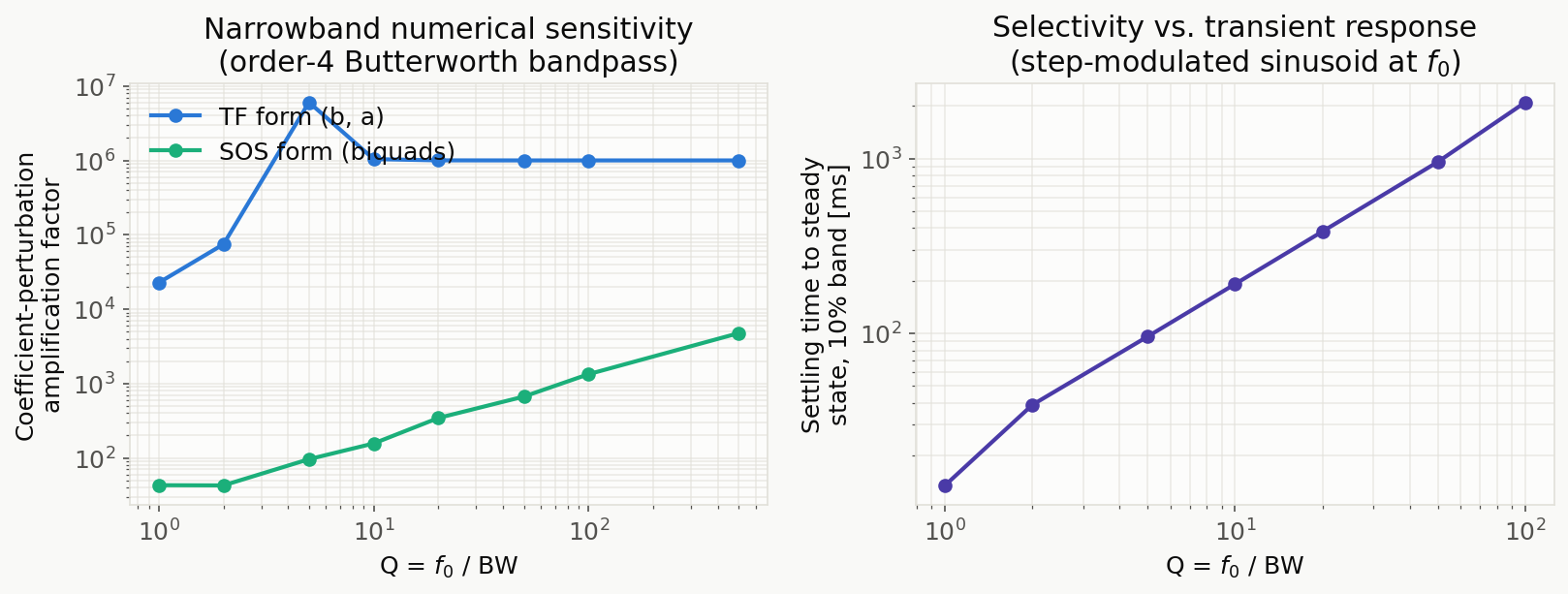
The figure above shows, on the left, the coefficient-perturbation sensitivity from this section (TF form vs. SOS form), and on the right, the Q-vs-settling-time relationship measured in the previous section. Both are close to straight lines on log-log axes, visually confirming that the numerical difficulty and the slowness of the transient response both worsen with a power-law dependence on Q.
Practical mitigations: use the SOS form (scipy.signal.butter(..., output='sos')), avoid raising the order unnecessarily, avoid making the bandwidth extremely narrow relative to the center frequency when possible (a rough guideline is to keep Q ≲ 100), and consider other numerically robust realizations such as state-space or lattice structures.
Python Implementation
IIR Bandpass Filter with scipy.signal
import numpy as np
import matplotlib.pyplot as plt
from scipy import signal

# --- Parameters ---
fs = 1000.0          # Sampling frequency [Hz]
f_low = 50.0         # Lower cutoff [Hz]
f_high = 150.0       # Upper cutoff [Hz]
order = 4            # Filter order

# --- Design Butterworth bandpass filter ---
nyq = fs / 2.0
low = f_low / nyq
high = f_high / nyq

b, a = signal.butter(order, [low, high], btype='bandpass')

# --- Compute frequency response ---
w, h = signal.freqz(b, a, worN=8000, fs=fs)

# --- Plot ---
fig, (ax1, ax2) = plt.subplots(2, 1, figsize=(10, 8))

# Gain (dB)
ax1.semilogx(w, 20 * np.log10(np.abs(h) + 1e-10))
ax1.axvline(f_low, color='r', linestyle='--', label=f'$f_l$ = {f_low} Hz')
ax1.axvline(f_high, color='g', linestyle='--', label=f'$f_h$ = {f_high} Hz')
ax1.axhline(-3, color='gray', linestyle=':', label='-3 dB')
ax1.set_xlabel('Frequency [Hz]')
ax1.set_ylabel('Gain [dB]')
ax1.set_title(f'Butterworth Bandpass Filter (order={order})')
ax1.legend()
ax1.grid(True, which='both', alpha=0.3)
ax1.set_xlim([1, nyq])
ax1.set_ylim([-80, 5])

# Phase
ax2.semilogx(w, np.angle(h, deg=True))
ax2.axvline(f_low, color='r', linestyle='--')
ax2.axvline(f_high, color='g', linestyle='--')
ax2.set_xlabel('Frequency [Hz]')
ax2.set_ylabel('Phase [degrees]')
ax2.set_title('Phase Response')
ax2.grid(True, which='both', alpha=0.3)
ax2.set_xlim([1, nyq])

plt.tight_layout()
plt.savefig('bandpass_response.png', dpi=150, bbox_inches='tight')
plt.show()
FIR Bandpass Filter Design
IIR filters have nonlinear phase, but FIR filters can achieve linear phase. This is important in audio processing where phase distortion is audible.
from scipy.signal import firwin, freqz

# --- FIR bandpass filter ---
numtaps = 101        # Number of taps (odd number recommended)
fir_bpf = firwin(
    numtaps,
    [f_low, f_high],
    pass_zero=False,  # Bandpass specification
    fs=fs,
    window='hamming'
)

w_fir, h_fir = freqz(fir_bpf, worN=8000, fs=fs)

# IIR vs FIR comparison
plt.figure(figsize=(10, 5))
plt.semilogx(w, 20 * np.log10(np.abs(h) + 1e-10), label='IIR Butterworth (order=4)', linewidth=2)
plt.semilogx(w_fir, 20 * np.log10(np.abs(h_fir) + 1e-10), label=f'FIR Hamming (taps={numtaps})', linewidth=2, linestyle='--')
plt.axvline(f_low, color='r', linestyle=':', alpha=0.7, label=f'$f_l$ = {f_low} Hz')
plt.axvline(f_high, color='g', linestyle=':', alpha=0.7, label=f'$f_h$ = {f_high} Hz')
plt.axhline(-3, color='gray', linestyle=':', alpha=0.7)
plt.xlabel('Frequency [Hz]')
plt.ylabel('Gain [dB]')
plt.title('Bandpass Filter Comparison: IIR vs FIR')
plt.legend()
plt.grid(True, which='both', alpha=0.3)
plt.xlim([1, nyq])
plt.ylim([-80, 5])
plt.tight_layout()
plt.show()
Applying the Filter to a Signal
# --- Generate test signal ---
t = np.linspace(0, 1.0, int(fs), endpoint=False)

# Target signal: 100 Hz sine wave
signal_pure = np.sin(2 * np.pi * 100 * t)

# Noise: 10 Hz low-freq + 300 Hz high-freq + white noise
noise = (
    0.5 * np.sin(2 * np.pi * 10 * t) +
    0.5 * np.sin(2 * np.pi * 300 * t) +
    0.3 * np.random.randn(len(t))
)

x_noisy = signal_pure + noise

# --- Apply filter ---
# lfilter: causal filter (real-time, has phase delay)
y_lfilter = signal.lfilter(b, a, x_noisy)

# filtfilt: zero-phase filter (offline, no phase delay)
y_filtfilt = signal.filtfilt(b, a, x_noisy)

# --- Comparison plot ---
fig, axes = plt.subplots(3, 1, figsize=(12, 8), sharex=True)

axes[0].plot(t[:200], x_noisy[:200], alpha=0.8, label='Noisy signal')
axes[0].set_ylabel('Amplitude')
axes[0].set_title('Input Signal (noisy)')
axes[0].legend()
axes[0].grid(True, alpha=0.3)

axes[1].plot(t[:200], y_lfilter[:200], color='orange', label='lfilter (causal)')
axes[1].plot(t[:200], signal_pure[:200], color='gray', linestyle='--', alpha=0.6, label='True signal')
axes[1].set_ylabel('Amplitude')
axes[1].set_title('After lfilter (with phase delay)')
axes[1].legend()
axes[1].grid(True, alpha=0.3)

axes[2].plot(t[:200], y_filtfilt[:200], color='green', label='filtfilt (zero-phase)')
axes[2].plot(t[:200], signal_pure[:200], color='gray', linestyle='--', alpha=0.6, label='True signal')
axes[2].set_ylabel('Amplitude')
axes[2].set_xlabel('Time [s]')
axes[2].set_title('After filtfilt (zero-phase)')
axes[2].legend()
axes[2].grid(True, alpha=0.3)

plt.tight_layout()
plt.savefig('bandpass_filtering_result.png', dpi=150, bbox_inches='tight')
plt.show()
IIR vs FIR Design Comparison
| Property | IIR (Butterworth, etc.) | FIR |
|---|---|---|
| Phase response | Nonlinear (phase distortion) | Linear phase achievable |
| Number of coefficients | Small (\(2N+1\) approx.) | Large (tens to hundreds) |
| Computational cost | Low | High (depends on tap count) |
| Stability | Risk with high orders | Always stable |
| Stopband roll-off | Steep at low order | Improves with tap count |
| Group delay | Non-constant | Constant (\((N-1)/2\) samples) |
| Typical use | Real-time processing | Audio, medical signals |
Design guidelines:
- Low computational cost in real-time → IIR (Butterworth / Chebyshev)
- Linear phase required (audio, medical) → FIR (Hamming / Kaiser window)
- Offline processing, zero phase delay →
filtfilt(works with both IIR and FIR)
IIR vs. FIR Order Comparison for an Identical Spec
The comparison table above summarizes qualitative characteristics, but comparing the actual order/tap count required to meet an identical specification makes the trade-off much more concrete.
We found the minimum order/tap count for IIR (Butterworth / Chebyshev I / Chebyshev II / elliptic) and FIR (window method / Parks-McClellan) to meet the following spec (\(f_s=1000\) Hz):
- Passband: 50–150 Hz, passband ripple ≤ 1 dB
- Stopband: ≤ 30 Hz and ≥ 170 Hz, stopband attenuation ≥ 40 dB
- Transition width: 20 Hz on each side
Using scipy.signal.buttord / cheb1ord / cheb2ord / ellipord to find the minimum order meeting this spec gives:
| Design method | Minimum order (prototype) | Realized bandpass poles (order × 2) |
|---|---|---|
| Butterworth | 21 | 42 |
| Chebyshev Type I | 8 | 16 |
| Chebyshev Type II | 8 | 16 |
| Elliptic (Cauer) | 5 | 10 |
Even for the same spec, Butterworth’s insistence on a maximally flat passband requires a very high order (21, realized as 42 poles), while Chebyshev — which allows ripple in either the passband or stopband — only needs order 8, and elliptic — which allows ripple in both — needs as few as order 5. This confirms that when a sharp transition band is required, trading away maximal flatness for equiripple behavior is far more efficient (consistent with the ripple/roll-off trade-off discussed in Chebyshev Filter Design: Theory and Python Implementation ).
For FIR, estimating the required tap count with scipy.signal.kaiserord (Kaiser window) gave 113 taps (\(\beta=3.395\)
). However, actually checking the realized frequency response, the achieved passband ripple was 6.08 dB — far exceeding the 1 dB target (stopband attenuation of 47.8 dB on the low side and 45.8 dB on the high side did meet the target). This is because the Kaiser window design formula estimates the tap count approximately from stopband attenuation and transition width, and does not directly guarantee passband ripple.
By contrast, using the equiripple Parks-McClellan method (scipy.signal.remez) to search for the minimum tap count meeting the same spec found a solution at 107 taps, achieving a passband ripple of 0.17 dB and stopband attenuation of 40.0 dB (low) / 40.1 dB (high) — meeting the spec tightly with no wasted margin.
Three practical takeaways from this experiment:
- For IIR, the required order for the same spec varies enormously with the design method (maximally flat vs. equiripple). When a sharp transition band is required, it is worth considering Chebyshev or elliptic designs.
- FIR requires far more taps (around 100 here) than IIR’s order (5 to 21 in this example), so IIR is more efficient per-sample computationally. FIR’s advantage is exact linear phase.
- The windowed method is simple but can fail to precisely meet some specs (such as ripple). When exact spec compliance must be verified, the Parks-McClellan (equiripple) method is more reliable.
Effect of Filter Order
fig, ax = plt.subplots(figsize=(10, 6))

for ord_n in [2, 4, 6, 8]:
    b_n, a_n = signal.butter(ord_n, [low, high], btype='bandpass')
    w_n, h_n = signal.freqz(b_n, a_n, worN=8000, fs=fs)
    ax.semilogx(w_n, 20 * np.log10(np.abs(h_n) + 1e-10), label=f'order={ord_n}')

ax.axhline(-3, color='gray', linestyle=':', label='-3 dB')
ax.axvline(f_low, color='r', linestyle='--', alpha=0.5)
ax.axvline(f_high, color='g', linestyle='--', alpha=0.5)
ax.set_xlabel('Frequency [Hz]')
ax.set_ylabel('Gain [dB]')
ax.set_title('Effect of Filter Order on Bandpass Response')
ax.legend()
ax.grid(True, which='both', alpha=0.3)
ax.set_xlim([1, nyq])
ax.set_ylim([-80, 5])
plt.tight_layout()
plt.show()
Higher order yields steeper roll-off, but IIR filters become numerically unstable at very high orders. Order ≤ 8 is a practical guideline.
Recent Research Trends (2023 and Later)
Bandpass filters are a classical signal-processing element, but research in wireless communication and RF front ends remains active.
- On-chip adjustable RF bandpass filters: IEEE Microwave Magazine (January 2024) published a review of on-chip frequency-adjustable RF bandpass filters, surveying designs that let a single circuit electrically switch its center frequency for multiband radios and software-defined radio (SDR).
- Widely tunable microstrip bandpass filters: A 2024 paper in MDPI Electronics reports a compact microstrip bandpass filter whose center frequency can be continuously tuned from 1.1 to 3.1 GHz using only a single bias voltage, reflecting the need for reconfigurable RF front ends for the broadband, multiband operation demanded by standards such as 5G/6G.
- Machine-learning-driven filter design optimization: A 2025 paper in Physica Scripta reports a machine-learning-based approach to bandpass filter design and optimization, and a 2025 MDPI Electronics paper describes using machine-learning models such as XGBoost to predict coupling matrices and physical parameters for microwave filters, reducing the number of design iterations. In the digital IIR/FIR domain, metaheuristic techniques such as differential evolution and grey wolf optimization have also been used to optimize filter coefficients (e.g., a 2024 Scientific Reports paper).
A common thread across these developments is combining classical analytical design (such as the Butterworth transformation and window methods covered in this article) with tunability and machine-learning-driven design automation and acceleration. Note, however, that most of these techniques target microwave/RF circuits (analog hardware); directly applying ML optimization to digital-signal-processing bandpass filter design of the kind covered in this article remains, as of this writing, a less-developed area.
Related Articles
- Lowpass Filter Design: Moving Average, Butterworth, Chebyshev — LPF prototype design that forms the basis of bandpass filter design.
- Butterworth Filter Design: Theory and Python Implementation — The Butterworth LPF prototype used in bandpass design.
- FIR vs IIR Filters: A Comprehensive Comparison — Design philosophy differences between FIR and IIR filters.
- Chebyshev Filter Design: Theory and Python Implementation — Equiripple IIR prototype that yields a sharper bandpass transition than Butterworth at the same order.
- Notch Filter Design and Python Implementation — Band-stop (notch) filter that is the complement of a bandpass filter.
- Frequency Characteristics of the Exponential Moving Average Filter — EMA as a 1st-order IIR lowpass filter derived via Z-transform.
- FFT: Theory and Python Implementation — FFT fundamentals for verifying bandpass filter effects in the frequency domain.
- Window Functions and Power Spectral Density — Mathematical background of window functions used in FIR filter design.
- Adaptive Filters (LMS/RLS): Theory and Python Implementation — Filters that automatically adjust their frequency response to the environment.
- Highpass Filter Design and Python Implementation — The HPF half that, combined with an LPF, forms a bandpass.
- Bessel Filter: Theory and Python Implementation — Maximally flat group delay IIR prototype, suitable when in-band phase linearity matters.
- Bode Plot: Theory and Python Implementation — Hub article for visualizing bandpass magnitude around the center frequency and the symmetric phase response.
- Hilbert Transform and the Analytic Signal: Theory and Python Implementation — Typical workflow: narrow the band first with a bandpass, then extract envelope and instantaneous phase via Hilbert.
- Filter Design Selection Guide: 3 axes and characteristic comparison — Use this hub to position the bandpass filter against alternatives during selection.
References
- Proakis, J. G., & Manolakis, D. G. (2006). Digital Signal Processing: Principles, Algorithms, and Applications. Pearson.
- scipy.signal.butter — SciPy documentation
- scipy.signal.filtfilt — SciPy documentation
- A Review of On-Chip Adjustable RF Bandpass Filters — IEEE Microwave Magazine, January 2024.
- A Compact Bandpass Filter with Widely Tunable Frequency and Simple Bias Control — Electronics (MDPI), 13(2), 411 (2024).
- Machine Learning-Driven Approaches for Advanced Microwave Filter Design — Electronics (MDPI), 14(2), 367 (2025).
- Design and optimization of a bandpass filter using machine learning — Physica Scripta, 100, 075574 (2025).
Related Tools
- DevToolBox - Free Developer Tools — 85+ tools including JSON formatter, regex tester
- CalcBox - Everyday Calculation Tools — 61+ tools including statistics and frequency conversion