What Is a Complementary Filter?
A complementary filter is a technique for optimally combining outputs from two sensors with different noise characteristics in the frequency domain. It applies a high-pass filter to one sensor and a low-pass filter to the other, designed so that their sum equals unity across all frequencies.
The most common application is sensor fusion of gyroscopes and accelerometers in an IMU (Inertial Measurement Unit).
| Sensor | Strength | Weakness |
|---|---|---|
| Gyroscope | Accurate for short-term changes | Drift accumulates over time |
| Accelerometer | Stable over long periods (gravity reference) | Sensitive to vibration and noise |
Gyroscopes compute angle by integrating angular velocity, so bias errors accumulate as drift (low-frequency error). Accelerometers can determine tilt from the gravity vector but are susceptible to vibration and translational acceleration (high-frequency noise).
The complementary filter exploits this complementary nature: it extracts high-frequency components from the gyroscope and low-frequency components from the accelerometer, canceling the weaknesses of both.
Key Application Areas
- Drones and multicopters: Attitude estimation (pitch and roll angles)
- Robotics: Posture stabilization for bipedal robots
- Smartphones: Screen rotation, AR/VR head tracking
- Vehicle control: Sideslip angle estimation
Theory
Complementarity of High-Pass and Low-Pass Filters
The core principle of the complementary filter is that the high-pass filter \(H_{HPF}(z)\) and low-pass filter \(H_{LPF}(z)\) satisfy the following relationship:
\[H_{HPF}(z) + H_{LPF}(z) = 1 \tag{1}\]This property ensures that the combined sensor output is reconstructed without distortion across the entire frequency band.
Transfer Function of a First-Order Complementary Filter
Define the first-order low-pass filter transfer function as:
\[H_{LPF}(z) = \frac{(1-\alpha)}{1 - \alpha z^{-1}} \tag{2}\]From the complementary condition \((1)\) , the high-pass filter becomes:
\[H_{HPF}(z) = 1 - H_{LPF}(z) = \frac{1 - z^{-1}}{1 - \alpha z^{-1}} \tag{3}\]The complementary filter output for gyroscope output \(X_{gyro}(z)\) and accelerometer output \(X_{accel}(z)\) is:
\[Y(z) = H_{HPF}(z) \cdot X_{gyro}(z) + H_{LPF}(z) \cdot X_{accel}(z) \tag{4}\]Time-Domain Update Equation
Taking the inverse Z-transform of equation \((4)\) yields the following recursive update equation:
\[\theta[n] = \alpha \left(\theta[n-1] + \dot{\theta}_{gyro}[n] \cdot \Delta t\right) + (1 - \alpha) \cdot \theta_{accel}[n] \tag{5}\]where:
- \(\theta[n]\) : Current estimated angle
- \(\dot{\theta}_{gyro}[n]\) : Gyroscope angular velocity output
- \(\theta_{accel}[n]\) : Angle computed from accelerometer
- \(\Delta t\) : Sampling period
- \(\alpha\) : Filter coefficient (\(0 < \alpha < 1\) )
Equation \((5)\) can be interpreted intuitively:
- First term: Weights the gyroscope integration by \(\alpha\) (high-pass filter effect)
- Second term: Weights the accelerometer angle by \((1-\alpha)\) (low-pass filter effect)
Relationship Between Time Constant \(\tau\) and Filter Coefficient \(\alpha\)
The parameter \(\alpha\) is determined from the time constant \(\tau\) and sampling period \(\Delta t\) :
\[\alpha = \frac{\tau}{\tau + \Delta t} \tag{6}\]The physical meaning of the time constant \(\tau\) is:
- Large \(\tau\) (\(\alpha \to 1\) ): Greater gyroscope contribution. Good short-term response but slow drift correction
- Small \(\tau\) (\(\alpha \to 0\) ): Greater accelerometer contribution. Fast drift correction but susceptible to vibration noise
The crossover frequency \(f_c\) (where LPF and HPF gains are equal) is:
\[f_c = \frac{1}{2\pi\tau} \tag{7}\]Equivalence With the Steady-State Kalman Filter: A Rigorous Derivation
Rather than simply asserting that “a first-order complementary filter is a special case of the steady-state Kalman filter,” we derive this starting from a scalar (1D) Kalman filter. Consider a scalar state-space model where the gyroscope angular rate \(\dot\theta_{gyro}[n]\) is the control input of the predict step and the accelerometer angle \(\theta_{accel}[n]\) is the observation.
Predict step:
\[\hat\theta^-[n] = \hat\theta[n-1] + \dot\theta_{gyro}[n] \cdot \Delta t, \qquad P^-[n] = P[n-1] + Q \tag{8}\]Here \(Q\) is the variance that gyroscope noise (standard deviation \(\sigma_g\) ) contributes to angular uncertainty after one step of integration, approximated as \(Q \approx (\sigma_g \Delta t)^2\) .
Update step:
\[K[n] = \frac{P^-[n]}{P^-[n] + R}, \qquad \hat\theta[n] = (1 - K[n])\,\hat\theta^-[n] + K[n]\,\theta_{accel}[n] \tag{9}\]Here \(R = \sigma_a^2\) is the accelerometer’s angle-referred noise variance. Setting \(\alpha := 1 - K[n]\) in equation \((9)\) makes it identical in form to the update equation \((5)\) (\(\hat\theta^-[n]\) corresponds to the first term’s gyro integration, and \(\theta_{accel}[n]\) to the second term). In other words, the complementary filter and the Kalman filter share the same update equation — the only difference is whether the gain \(\alpha\) (or \(K\) ) is fixed or time-varying.
Deriving the steady-state gain: If \(Q, R\) are time-invariant, the covariance \(P[n]\) converges to a fixed point \(P^*\) of the discrete Riccati equation. Substituting the steady-state condition \(P[n]=P[n-1]=P^*\) into equations \((8)(9)\) gives:
\[P^* = (1 - K^*)(P^* + Q), \qquad K^* = \frac{P^* + Q}{P^* + Q + R} \tag{10}\]Eliminating \(P^*\) from these two equations, and writing \(\alpha^* := 1 - K^*\) and the noise ratio \(r := Q/R\) , yields the following quadratic (derivation: from \(P^*=\alpha^*(P^*+Q)\) we get \(P^*+Q=P^*/\alpha^*\) ; substituting into the expression for \(K^*\) and using \(\alpha^*=1-K^*\) gives \(P^*=(1-\alpha^*)R\) ; equating the two and simplifying with \(r=Q/R\) ):
\[(\alpha^*)^2 - (2 + r)\,\alpha^* + 1 = 0 \tag{11}\]Selecting the root satisfying \(0 < \alpha^* < 1\) gives the closed-form solution:
\[\alpha^* = 1 + \frac{r}{2} - \sqrt{r + \frac{r^2}{4}} \tag{12}\]Equation \((12)\) shows that the complementary filter’s fixed parameter \(\alpha\) is mathematically equivalent to the steady-state Kalman filter only when it matches the gyro/accelerometer noise-variance ratio \(r=Q/R\) . In other words, manually tuning \(\alpha\) (or \(\tau\) ) in a complementary filter implicitly amounts to estimating this noise ratio. Combined with \(\tau = \alpha\Delta t/(1-\alpha)\) from equation \((6)\) , we can compute a theoretically optimal time constant \(\tau^*\) directly from the noise statistics \(\sigma_g, \sigma_a\) . We verify this theoretical prediction numerically against real data later, in “Effect of Parameter \(\alpha\) .”
Note that this derivation models \(Q\) as zero-mean process noise and does not account for gyroscope bias (a non-zero-mean systematic error). For real sensors with bias, equation \((12)\) ’s prediction is valid only as a theoretical upper bound — the actual optimal \(\tau\) shifts smaller due to the bias. We examine this in detail in the edge cases section below.
Frequency Response Analysis
Analyzing the complementary filter’s frequency response confirms that the LPF and HPF gains cross at the crossover frequency \(f_c\) , and their sum remains at 0 dB across all frequencies.
import numpy as np
import matplotlib.pyplot as plt
from scipy import signal

# --- Parameters ---
fs = 100.0           # Sampling frequency [Hz]
dt = 1.0 / fs
tau = 1.0            # Time constant [s]
alpha = tau / (tau + dt)

BLUE, ORANGE, RED = '#2a78d6', '#eb6834', '#e34948'  # categorical palette

# --- Transfer function definition ---
# LPF: H_LPF(z) = (1-alpha) / (1 - alpha*z^{-1})
b_lpf = [1 - alpha]
a_lpf = [1, -alpha]

# HPF: H_HPF(z) = (1 - z^{-1}) / (1 - alpha*z^{-1})
b_hpf = [1, -1]
a_hpf = [1, -alpha]

# --- Frequency response ---
w_lpf, h_lpf = signal.freqz(b_lpf, a_lpf, worN=4096, fs=fs)
w_hpf, h_hpf = signal.freqz(b_hpf, a_hpf, worN=4096, fs=fs)

# Combined frequency response
h_sum = h_lpf + h_hpf

fc = 1.0 / (2 * np.pi * tau)  # Crossover frequency

# --- Plot ---
fig, (ax1, ax2) = plt.subplots(2, 1, figsize=(10, 8))

# Gain characteristics
ax1.semilogx(w_lpf, 20 * np.log10(np.abs(h_lpf) + 1e-10),
             label='LPF (Accelerometer)', linewidth=2, color=BLUE)
ax1.semilogx(w_hpf, 20 * np.log10(np.abs(h_hpf) + 1e-10),
             label='HPF (Gyroscope)', linewidth=2, color=ORANGE)
ax1.semilogx(w_lpf, 20 * np.log10(np.abs(h_sum) + 1e-10),
             label='Sum (HPF + LPF)', linewidth=2, linestyle='--', color='black')
ax1.axvline(fc, color=RED, linestyle=':', alpha=0.8,
            label=f'$f_c$ = {fc:.3f} Hz')
ax1.axhline(-3, color='gray', linestyle=':', alpha=0.5, label='-3 dB')
ax1.set_xlabel('Frequency [Hz]')
ax1.set_ylabel('Gain [dB]')
ax1.set_title(f'Complementary Filter Frequency Response (τ={tau} s, α={alpha:.4f})')
ax1.legend()
ax1.grid(True, which='both', alpha=0.3)
ax1.set_xlim([0.001, fs / 2])
ax1.set_ylim([-40, 5])

# Phase characteristics
ax2.semilogx(w_lpf, np.angle(h_lpf, deg=True), label='LPF', linewidth=2, color=BLUE)
ax2.semilogx(w_hpf, np.angle(h_hpf, deg=True), label='HPF', linewidth=2, color=ORANGE)
ax2.axvline(fc, color=RED, linestyle=':', alpha=0.8)
ax2.set_xlabel('Frequency [Hz]')
ax2.set_ylabel('Phase [degrees]')
ax2.set_title('Phase Response')
ax2.legend()
ax2.grid(True, which='both', alpha=0.3)
ax2.set_xlim([0.001, fs / 2])

plt.tight_layout()
plt.savefig('complementary_frequency_response.png', dpi=150, bbox_inches='tight')
plt.show()
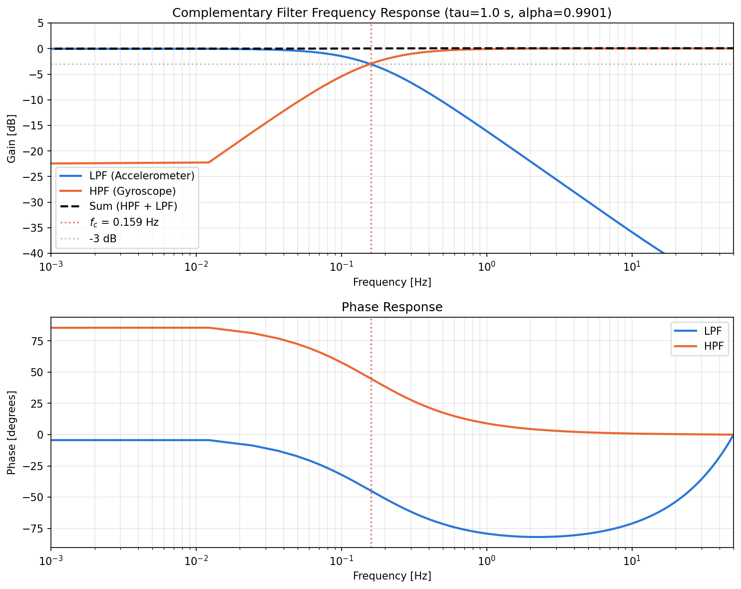
Running this with \(\tau = 1.0\) s gives \(\alpha = 0.9901\) and a crossover frequency \(f_c = 0.159\) Hz. The LPF and HPF gains cross at \(-3\) dB at this frequency, and their sum (black dashed line) stays at 0 dB (= 1) across all frequencies — this is why the filter is called “complementary.” The phase plot shows the LPF and HPF phases swinging with opposite sign and near-symmetric magnitude around the crossover frequency, confirming that the cancellation holds in phase as well as amplitude.
Python Implementation
IMU Sensor Simulation
We simulate realistic IMU sensors to verify the complementary filter’s effectiveness.
import numpy as np
import matplotlib.pyplot as plt

np.random.seed(42)  # fix the seed for reproducibility

BLUE, ORANGE, GREEN, RED = '#2a78d6', '#eb6834', '#1baf7a', '#e34948'

# --- Simulation parameters ---
fs = 100.0           # Sampling frequency [Hz]
dt = 1.0 / fs
T = 30.0             # Simulation duration [s]
t = np.arange(0, T, dt)
N = len(t)

# --- True angle (test signal) ---
# Slow sinusoidal motion + step change
theta_true = (
    15.0 * np.sin(2 * np.pi * 0.1 * t) +     # 0.1 Hz oscillation
    5.0 * np.sin(2 * np.pi * 0.5 * t) +       # 0.5 Hz oscillation
    10.0 * (t > 15)                             # Step change at t=15s
)

# --- True angular velocity ---
omega_true = np.gradient(theta_true, dt)

# --- Gyroscope output (angular velocity + bias drift + noise) ---
gyro_bias = 0.5      # Bias [deg/s] (cause of drift)
gyro_noise_std = 2.0  # Noise standard deviation [deg/s]

gyro_output = omega_true + gyro_bias + gyro_noise_std * np.random.randn(N)

# --- Accelerometer output (angle + vibration noise) ---
accel_noise_std = 5.0  # Noise standard deviation [deg]

accel_output = theta_true + accel_noise_std * np.random.randn(N)

# --- Gyro-only angle estimation (integration) ---
theta_gyro = np.zeros(N)
theta_gyro[0] = theta_true[0]
for i in range(1, N):
    theta_gyro[i] = theta_gyro[i - 1] + gyro_output[i] * dt

# --- Complementary filter ---
tau = 1.0            # Time constant [s]
alpha = tau / (tau + dt)

theta_comp = np.zeros(N)
theta_comp[0] = theta_true[0]
for i in range(1, N):
    # Implementation of equation (5)
    theta_comp[i] = alpha * (theta_comp[i - 1] + gyro_output[i] * dt) \
                  + (1 - alpha) * accel_output[i]

# --- Comparison plot ---
fig, axes = plt.subplots(4, 1, figsize=(12, 14), sharex=True)

# True angle
axes[0].plot(t, theta_true, 'k-', linewidth=2, label='True angle')
axes[0].set_ylabel('Angle [deg]')
axes[0].set_title('True Angle')
axes[0].legend()
axes[0].grid(True, alpha=0.3)

# Gyro only
axes[1].plot(t, theta_gyro, color=ORANGE, alpha=0.9, label='Gyro only (integration)')
axes[1].plot(t, theta_true, 'k--', alpha=0.5, label='True')
axes[1].set_ylabel('Angle [deg]')
axes[1].set_title('Gyroscope Only (drift accumulation)')
axes[1].legend()
axes[1].grid(True, alpha=0.3)

# Accelerometer only
axes[2].plot(t, accel_output, color=BLUE, alpha=0.6, label='Accelerometer only')
axes[2].plot(t, theta_true, 'k--', alpha=0.5, label='True')
axes[2].set_ylabel('Angle [deg]')
axes[2].set_title('Accelerometer Only (noisy)')
axes[2].legend()
axes[2].grid(True, alpha=0.3)

# Complementary filter
axes[3].plot(t, theta_comp, color=GREEN, linewidth=2, label=f'Complementary (α={alpha:.3f})')
axes[3].plot(t, theta_true, 'k--', alpha=0.5, label='True')
axes[3].set_ylabel('Angle [deg]')
axes[3].set_xlabel('Time [s]')
axes[3].set_title('Complementary Filter')
axes[3].legend()
axes[3].grid(True, alpha=0.3)

plt.tight_layout()
plt.savefig('complementary_filter_comparison.png', dpi=150, bbox_inches='tight')
plt.show()

# --- RMSE calculation ---
rmse_gyro = np.sqrt(np.mean((theta_gyro - theta_true) ** 2))
rmse_accel = np.sqrt(np.mean((accel_output - theta_true) ** 2))
rmse_comp = np.sqrt(np.mean((theta_comp - theta_true) ** 2))

print(f"RMSE (Gyro only):          {rmse_gyro:.2f} deg")
print(f"RMSE (Accelerometer only): {rmse_accel:.2f} deg")
print(f"RMSE (Complementary):      {rmse_comp:.2f} deg")
Running with seed=42 gives the following measured results:
RMSE (Gyro only):          9.79 deg
RMSE (Accelerometer only): 5.05 deg
RMSE (Complementary):      0.53 deg
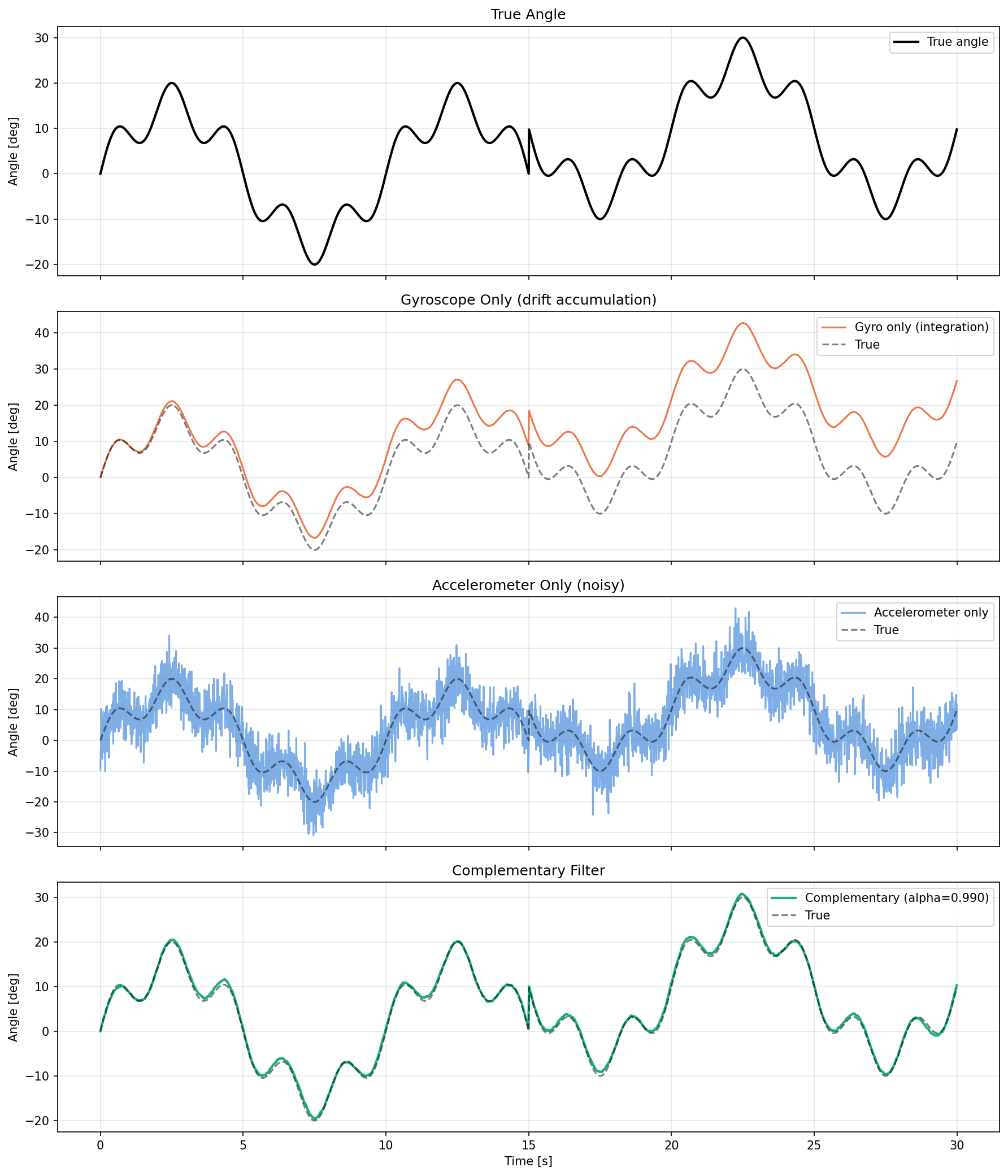
The gyro-only estimate (RMSE 9.79°) diverges significantly from the true value over time due to bias drift, while the accelerometer-only estimate (RMSE 5.05°) fluctuates heavily due to vibration noise. The complementary filter (RMSE 0.53°) mitigates both issues, reducing RMSE to roughly 1/18 of the gyro-only value and about 1/9.5 of the accelerometer-only value. In the fourth panel, the complementary filter’s output (green) nearly overlaps the true value (gray dashed), tracking the step change at \(t=15\) s without significant overshoot.
Effect of Parameter \(\alpha\)
We analyze how different values of \(\alpha\) (time constant \(\tau\) ) affect estimation accuracy.
# --- Comparison with different α (τ) values ---
tau_values = [0.1, 0.5, 1.0, 5.0, 10.0]
colors = [BLUE, ORANGE, GREEN, '#4a3aa7', RED]

fig, axes = plt.subplots(2, 1, figsize=(12, 10))

for tau_val, c in zip(tau_values, colors):
    alpha_val = tau_val / (tau_val + dt)
    theta_est = np.zeros(N)
    theta_est[0] = theta_true[0]
    for i in range(1, N):
        theta_est[i] = alpha_val * (theta_est[i - 1] + gyro_output[i] * dt) \
                      + (1 - alpha_val) * accel_output[i]

    rmse = np.sqrt(np.mean((theta_est - theta_true) ** 2))
    axes[0].plot(t, theta_est, color=c, label=f'τ={tau_val}s (α={alpha_val:.4f}, RMSE={rmse:.2f}°)')

axes[0].plot(t, theta_true, 'k--', linewidth=2, alpha=0.7, label='True')
axes[0].set_ylabel('Angle [deg]')
axes[0].set_xlabel('Time [s]')
axes[0].set_title('Effect of Time Constant τ on Complementary Filter')
axes[0].legend(fontsize=8)
axes[0].grid(True, alpha=0.3)

# τ vs RMSE plot
tau_range = np.logspace(-2, 2, 100)
rmse_list = []
for tau_val in tau_range:
    alpha_val = tau_val / (tau_val + dt)
    theta_est = np.zeros(N)
    theta_est[0] = theta_true[0]
    for i in range(1, N):
        theta_est[i] = alpha_val * (theta_est[i - 1] + gyro_output[i] * dt) \
                      + (1 - alpha_val) * accel_output[i]
    rmse_list.append(np.sqrt(np.mean((theta_est - theta_true) ** 2)))

axes[1].semilogx(tau_range, rmse_list, color=BLUE, linewidth=2)
axes[1].set_xlabel('Time Constant τ [s]')
axes[1].set_ylabel('RMSE [deg]')
axes[1].set_title('RMSE vs Time Constant τ')
axes[1].grid(True, which='both', alpha=0.3)

# Empirically found optimal τ
optimal_idx = np.argmin(rmse_list)
optimal_tau = tau_range[optimal_idx]
optimal_rmse = rmse_list[optimal_idx]
axes[1].axvline(optimal_tau, color=RED, linestyle='--',
                label=f'Empirical optimal τ={optimal_tau:.2f}s (RMSE={optimal_rmse:.2f}°)')

# Analytic τ* from equation (12) (assumes zero-mean noise only, ignores bias)
Q = (gyro_noise_std * dt) ** 2   # variance from one-step gyro noise integration
R = accel_noise_std ** 2         # accelerometer angle-referred variance
r = Q / R
alpha_star = 1 + r / 2 - np.sqrt(r ** 2 / 4 + r)
tau_star = alpha_star * dt / (1 - alpha_star)
axes[1].axvline(tau_star, color='#4a3aa7', linestyle=':',
                label=f'Analytic τ*={tau_star:.2f}s (noise-only, bias ignored)')
axes[1].legend(fontsize=8)

plt.tight_layout()
plt.savefig('alpha_effect.png', dpi=150, bbox_inches='tight')
plt.show()

print(f"Q={Q:.6f} deg^2, R={R:.3f} deg^2, r=Q/R={r:.8f}")
print(f"Empirical optimal tau = {optimal_tau:.4f} s (RMSE={optimal_rmse:.3f} deg)")
print(f"Analytic alpha* = {alpha_star:.6f}, tau* = {tau_star:.4f} s")
The seed=42 run produces:
Q=0.000400 deg^2, R=25.000 deg^2, r=Q/R=0.00001600
Empirical optimal tau = 0.7221 s (RMSE=0.493 deg)
Analytic alpha* = 0.996008, tau* = 2.4950 s
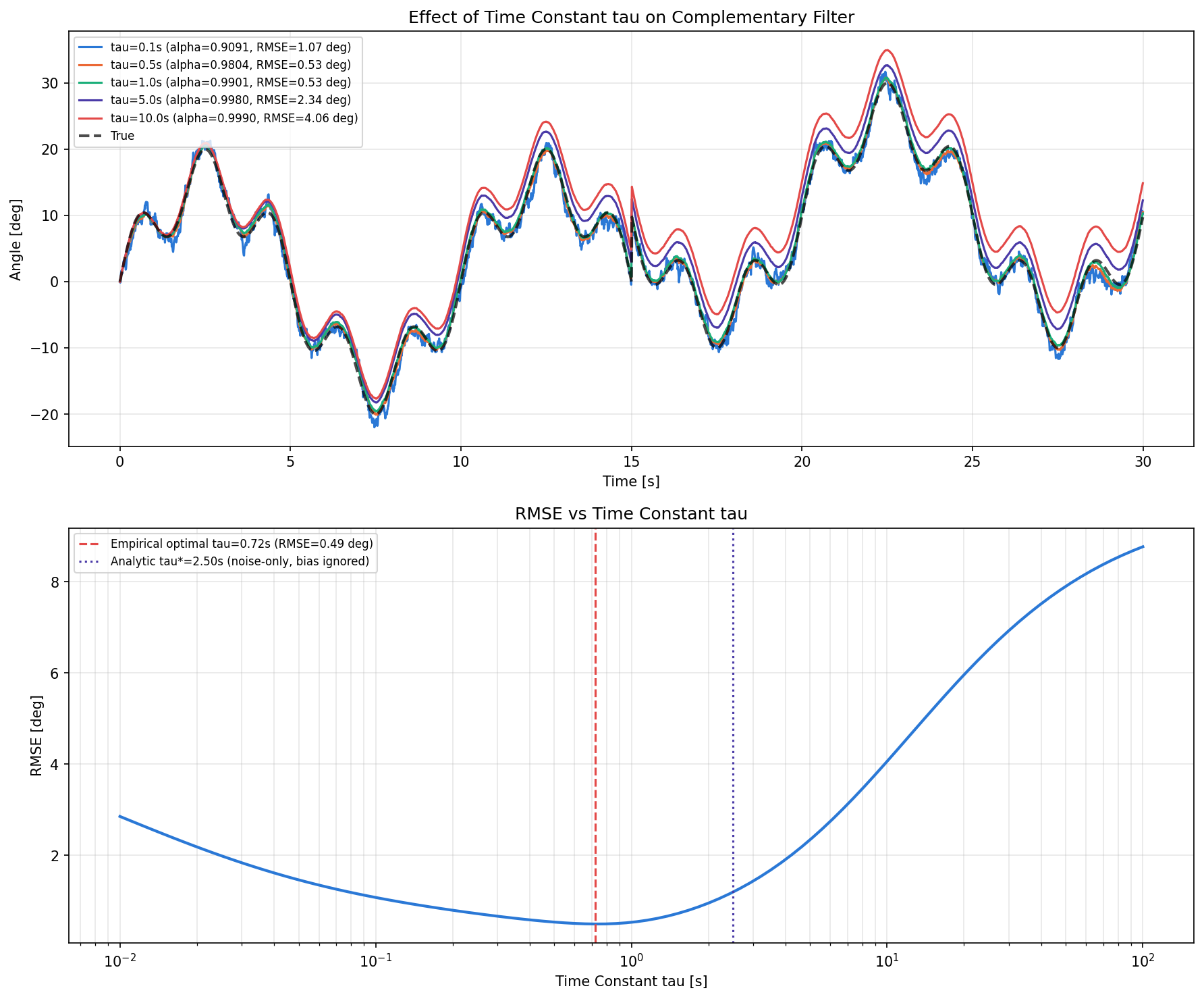
The empirically found optimal time constant is \(\tau \approx 0.72\)
s (RMSE 0.49°), but the analytic optimum predicted by equation \((12)\)
is \(\tau^* \approx 2.50\)
s — the two do not match. This is not an error in the theory: the derivation in equations \((8)\)
–\((12)\)
assumes zero-mean process noise only and does not account for the \(0.5\)
deg/s systematic gyro bias present in the simulation. Indeed, re-running the same sweep with gyro_bias = 0 pushes the empirical optimum up to \(2.97\)
s, much closer to the analytic value of \(2.50\)
s (same conditions, seed=42). When bias is present, increasing \(\tau\)
(trusting the gyro more) accumulates more bias-driven error through integration, so the practically useful \(\tau\)
is smaller than the value predicted from noise statistics alone. This finding connects directly to the edge case discussed below: gyroscope bias violates the assumptions behind the complementary filter / steady-state Kalman filter equivalence.
Guidelines for choosing \(\alpha\) :
| \(\tau\) Range | \(\alpha\) Tendency | Characteristics |
|---|---|---|
| \(\tau < 0.5\) s | Small \(\alpha\) | Accelerometer-weighted. More noise but less drift |
| \(0.5 \le \tau \le 2\) s | Medium \(\alpha\) | Balanced. Suitable for most applications |
| \(\tau > 5\) s | Large \(\alpha\) | Gyroscope-weighted. Good response but more drift |
The optimal \(\tau\) depends on the sensor noise characteristics. If the gyroscope bias is large, use a smaller \(\tau\) ; if the accelerometer noise is large, use a larger \(\tau\) (equation \((12)\) should be treated as an upper-bound guideline for the ideal, bias-free case — always validate numerically against real data).
Comparison with Kalman Filter
Both complementary filters and Kalman filters are used for sensor fusion, but they differ in design philosophy.
| Property | Complementary Filter | Kalman Filter |
|---|---|---|
| Parameters | \(\alpha\) (single) | \(Q, R, P\) (process and observation noise covariance) |
| Computational cost | Very low (add/multiply only) | Moderate (matrix operations) |
| Design complexity | Simple | Requires model definition |
| Optimality | Not optimal | Optimal under linear Gaussian assumptions |
| Adaptivity | Fixed parameters | Gain auto-adjusts |
| Nonlinear systems | Not supported | EKF/UKF available |
| Real-time suitability | Extremely high | High (embedded implementations exist) |
| Lines of code | ~5 lines | ~30-50 lines |
Selection guidelines:
- Resource-constrained microcontrollers (Arduino, etc.) — Complementary filter
- Known noise characteristics requiring optimal estimation — Kalman filter
- Prototyping and educational purposes — Complementary filter (easier to understand)
- Multi-sensor fusion (GPS + IMU, etc.) — Kalman filter
In fact, a first-order complementary filter can be viewed as a special case of the steady-state Kalman filter. We derived this rigorously in equations \((8)\) –\((12)\) in the Theory section, and showed that a theoretically optimal time constant \(\tau^*\) can be computed from noise statistics. However, as confirmed numerically above (see “Effect of Parameter \(\alpha\) ”), gyroscope bias in realistic conditions causes the analytic value to diverge from the empirical optimum, so real deployments should always combine the theory with numerical tuning.
Edge Cases and Implementation Pitfalls
The complementary filter’s simplicity comes with several pitfalls and applicability limits worth knowing.
Gyroscope Bias Violates the Theory’s Assumptions
The steady-state Kalman equivalence derived in equations \((8)\) –\((12)\) models the process noise \(Q\) as zero-mean. Real MEMS gyroscopes, however, exhibit temperature-dependent systematic bias, which grows into drift proportional to time once integrated. As seen in the “Effect of Parameter \(\alpha\) ” numerical experiment, a bias of \(0.5\) deg/s pushes the numerically optimal time constant (\(\tau\approx0.72\) s) far below the bias-free theoretical value (\(\tau^*\approx2.50\) s). When bias is unknown or time-varying, a complementary filter alone cannot cancel it out — consider pre-calibration or a bias-augmented Kalman filter / complementary filter that estimates bias as an additional state variable.
Handling Variable Sampling Periods (Jitter)
Equation \((6)\) ’s \(\alpha = \tau/(\tau+\Delta t)\) assumes a fixed \(\Delta t\) . In embedded systems, task-scheduling delays commonly cause \(\Delta t\) to vary from one loop iteration to the next (jitter). Computing \(\alpha\) once at startup and holding it fixed breaks the complementary property (\(H_{HPF}+H_{LPF}=1\) ) whenever \(\Delta t\) fluctuates. In practice, measure the actual \(\Delta t_n\) each loop iteration and recompute \(\alpha_n = \tau/(\tau+\Delta t_n)\) every time.
Angle Wraparound (±180° Boundary)
Applying the simple linear-interpolation update in equation \((5)\)
directly to a quantity that wraps discontinuously at \(\pm 180°\)
, such as yaw, causes a false \(358°\)
error the instant the true angle crosses from \(179°\)
to \(-179°\)
, sending the filter into a runaway state. The fix is to normalize the angle difference to \((-180°, 180°]\)
— e.g. via atan2(sin(Δθ), cos(Δθ)) — before applying equation \((5)\)
, or to switch to a quaternion representation as discussed below. Our simulation deliberately stays within roughly \(\pm 30°\)
to sidestep this issue.
Accelerometers Cannot Distinguish Gravity From Translational Acceleration
The tilt-angle formula computed from accelerometer data assumes the sensed acceleration vector is gravity alone. When a vehicle or drone undergoes translational acceleration (hard braking, sharp turns), the accelerometer output deviates from the gravity direction, introducing a systematic error into the tilt estimate. A low-pass filter cannot fully remove this error — if the translational-acceleration frequency content overlaps below the crossover frequency \(f_c\) , it passes through as a low-frequency attitude error. High-dynamics applications need an additional correction using GPS velocity or airspeed-sensor-derived translational acceleration.
Extending Beyond Roll/Pitch to 3D Attitude, and Gimbal Lock
Equation \((5)\) in this article targets a single-axis (roll or pitch) scalar angle. Handling full 3-axis attitude (roll, pitch, yaw) with Euler angles in a complementary filter suffers from gimbal lock — roll and yaw become indistinguishable as pitch approaches \(\pm 90°\) . In practice, attitude is represented with quaternions or rotation matrices: the gyro angular rate is integrated via the quaternion kinematic differential equation, and the result is complementarily corrected against the accelerometer- (and magnetometer-) derived attitude using spherical linear interpolation (SLERP) or a nonlinear feedback law such as the Mahony/Madgwick filter (see Mahony et al. 2008 in the references, a representative example).
Yaw Cannot Be Observed From the Accelerometer Alone
Since the accelerometer only senses the direction of gravity (the vertical axis), it cannot supply a low-frequency reference for yaw, which is rotation about the vertical axis. Correcting yaw drift requires a separate absolute reference such as a magnetometer (compass), GPS heading, or visual odometry. The 9-axis IMU configurations in the “Practical Applications” table address exactly this constraint.
Long-Term Drift From Floating-Point Arithmetic
Running the recursive update in equation \((5)\) in single precision (float32) over many hours or days can accumulate rounding error, producing a slow drift that the theoretical RMSE analysis does not account for. Long-running embedded deployments should use double precision (float64) where possible, or periodically reset to a known reference attitude.
Recent Research Trends
The limitations of a fixed parameter \(\alpha\) — notably the gyro-bias problem and the motion-dependent optimal \(\tau\) discussed above — have motivated recent work mainly in the direction of making the gain adapt to the situation.
- Jiang, P., Liu, C., Cong, H., & Zhang, F. (2024). A fuzzy adaptive complementary filter for attitude estimation based on norm judgment. Measurement and Control. This work feeds the deviation of the accelerometer, magnetometer, and gyroscope norms from their nominal values into a fuzzy inference system, switching the complementary filter’s gain online according to the motion state (static, low-dynamics, high-dynamics). This is a practical answer to exactly the problem this article demonstrated numerically: the optimal \(\tau\) shifts from its theoretical value depending on bias and motion state.
- Yamagishi, S., & Jing, L. (2026). Quaternion-Averaging-Based Adaptive Complementary Filter for Pedestrian Dead Reckoning With a Foot-Mounted AHRS. arXiv preprint arXiv:2607.05451. This complementary filter for a foot-mounted AHRS (Attitude and Heading Reference System) combines quaternion averaging — a more rigorous way of blending attitudes than linear interpolation — with adaptive weighting based on walking phase and magnetic-disturbance magnitude. It reports low error competitive with Kalman-filter-family methods at a lower computational cost, making it a recent real-world example that combines both gimbal-lock avoidance (via quaternions) and adaptive gain in a deployable system.
Both directions preserve the complementary filter’s key advantage — low computational cost — while addressing the weakness we confirmed numerically in this article: a fixed \(\alpha\) cannot track changes in motion state or sensor characteristics.
Practical Applications
| Application | Fused Sensors | Typical \(\tau\) | Notes |
|---|---|---|---|
| Drone attitude control | Gyro + Accelerometer | 0.5–2 s | Pitch and roll angle estimation |
| Smartphone screen rotation | Gyro + Accelerometer | 0.2–1 s | Balance between responsiveness and stability |
| Vehicle yaw rate estimation | Gyro + GPS heading | 1–5 s | Compensates GPS low sample rate |
| Robot attitude estimation | Gyro + Accelerometer + Magnetometer | 0.5–2 s | 9-axis IMU for yaw angle estimation |
| Pedestrian dead reckoning | Gyro + Accelerometer + Barometer | 1–3 s | Indoor positioning attitude estimation |
| VR/AR head tracking | Gyro + Accelerometer + Camera | 0.1–0.5 s | Low latency is critical |
Related Articles
- Low-Pass Filter Design and Comparison: Moving Average, Butterworth, and Chebyshev - Covers the theoretical background of the LPF component in complementary filters.
- High-Pass Filter Design and Python Implementation - Covers the theoretical background of the HPF component in complementary filters.
- Kalman Filter Theory and Python Implementation - Explains the Kalman filter, positioned as a more advanced alternative to complementary filters.
- Frequency Characteristics of the Exponential Moving Average (EMA) Filter - The LPF part of the complementary filter is equivalent to EMA; this article explains its frequency characteristics.
- Adaptive Filter (LMS/RLS) Theory and Python Implementation - Covers adaptive filters that automatically adjust parameters based on the environment.
- Bandpass Filter Design and Python Implementation - Combines the LPF+HPF separation of a complementary filter into a single band-selecting design.
- Bessel Filter: Theory and Python Implementation - Maximally flat group delay IIR design; useful as the LPF/HPF prototype when phase distortion must be minimized.
- Wiener Filter: Optimal Linear Filtering Theory and Python Implementation - The complementary filter can be viewed as an intuitive special case of the SNR-driven Wiener filter.
- Filter Design Selection Guide: 3 axes and characteristic comparison — Use this hub to position the complementary filter against alternatives during selection.
References
- Mahony, R., Hamel, T., & Pflimlin, J.-M. (2008). Nonlinear Complementary Filters on the Special Orthogonal Group. IEEE Transactions on Automatic Control, 53(5), 1203-1218.
- Higgins, W. T. (1975). A Comparison of Complementary and Kalman Filtering. IEEE Transactions on Aerospace and Electronic Systems, AES-11(3), 321-325.
- Jiang, P., Liu, C., Cong, H., & Zhang, F. (2024). A fuzzy adaptive complementary filter for attitude estimation based on norm judgment. Measurement and Control. https://doi.org/10.1177/00202940241227069
- Yamagishi, S., & Jing, L. (2026). Quaternion-Averaging-Based Adaptive Complementary Filter for Pedestrian Dead Reckoning With a Foot-Mounted AHRS. arXiv preprint arXiv:2607.05451. https://arxiv.org/abs/2607.05451
- Arduino and MPU6050 Accelerometer and Gyroscope Tutorial
Related Tools
- DevToolBox - Free Developer Tools - Over 85 developer tools including JSON formatter, regex tester, and more
- CalcBox - Everyday Calculation Tools - Over 61 calculation tools including statistics, frequency conversion, and more