What Is a Highpass Filter?
A highpass filter (HPF) passes frequency components above a specified cutoff frequency and attenuates components below it.
Applications include DC removal from audio signals, drift suppression in vibration sensors, and edge enhancement in image processing.
Key Parameters
| Parameter | Description |
|---|---|
| \(f_c\) | Cutoff frequency (-3 dB point) |
| \(\omega_c\) | Cutoff angular frequency (\(\omega_c = 2\pi f_c\) ) |
| \(N\) | Filter order (higher = steeper roll-off) |
| Passband | Frequency range \(f > f_c\) |
| Stopband | Frequency range \(f < f_c\) |
A higher order \(N\) yields a steeper roll-off, but also increases phase delay and the risk of numerical instability.
Frequency Response Derivation
Lowpass-to-Highpass Transformation
A highpass filter can be designed from a lowpass prototype (LPF) via a frequency transformation. In the analog domain, replace the complex variable \(s\) as:
\[ s \rightarrow \frac{\omega_c^2}{s} \tag{1}\]Applying transformation \((1)\) to the \(N\) th-order Butterworth LPF:
\[H_{LP}(s) = \frac{1}{\prod_{k=1}^{N}(s - s_k)} \tag{2}\]yields a Butterworth highpass filter of the same order. For the 1st-order case:
\[H_{HP}(s) = \frac{s}{s + \omega_c} \tag{3}\]Equation \((3)\) has a “differentiator + 1st-order lowpass” structure: output approaches zero as \(s \to 0\) (DC) and approaches 1 as \(s \to \infty\) (high frequency).
Why the Frequency Axis Gets Inverted (Deriving the Transformation)
Let’s derive why transformation \((1)\) produces a highpass response, by examining the correspondence on the frequency axis. Substituting \(s = j\omega\) into \((1)\) :
\[ j\omega \;\longrightarrow\; \frac{\omega_c^2}{j\omega} = -j\frac{\omega_c^2}{\omega} = j\left(-\frac{\omega_c^2}{\omega}\right) \]So a real frequency \(\omega\) is mapped to a new frequency \(\omega' = -\omega_c^2/\omega\) . Because the lowpass prototype’s transfer function has real coefficients (its impulse response is real-valued), the magnitude response is an even function of frequency: \(|H_{LP}(j\omega)| = |H_{LP}(-j\omega)|\) . Ignoring the sign, this gives
\[ |H_{HP}(j\omega)| = \left| H_{LP}\!\left(j\,\frac{\omega_c^2}{\omega}\right) \right| \]In words: the magnitude of the highpass response at frequency \(\omega\) equals the magnitude of the lowpass prototype’s response at frequency \(\omega_c^2/\omega\) .
- As \(\omega \to 0\) (DC), \(\omega_c^2/\omega \to \infty\) , which corresponds to the lowpass prototype’s fully-attenuated stopband — hence \(H_{HP}(0) = 0\) .
- As \(\omega \to \infty\) (high frequency), \(\omega_c^2/\omega \to 0\) , which corresponds to the lowpass prototype’s passband center (unity gain) — hence \(H_{HP}(j\infty) \to 1\) .
In other words, transformation \((1)\) folds the frequency axis via the inverse relation \(\omega \leftrightarrow \omega_c^2/\omega\) , swapping the lowpass prototype’s passband and stopband to create the highpass response. \(\omega = \omega_c\) is the fixed point of this fold (\(\omega_c^2/\omega_c = \omega_c\) ), which is also why the -3 dB points of both prototypes coincide.
Let’s verify this derivation numerically. We obtain the poles of a 4th-order Butterworth lowpass prototype (normalized to \(\omega_c = 1\)
) via scipy.signal.buttap, apply \(s \to \omega_c^2/s\)
by hand, and compare the result against what scipy.signal.lp2hp returns.
import numpy as np
from scipy import signal

N = 4
wc = 2 * np.pi * 100.0  # rad/s, fc = 100 Hz

# Normalized lowpass prototype (wc=1) poles
z_lp, p_lp, k_lp = signal.buttap(N)

# Lowpass poles scaled to wc
p_lp_scaled = p_lp * wc

# Manual transform: wc^2/s = p_lp  =>  s = wc^2 / p_lp
p_hp_manual = wc**2 / p_lp_scaled

# scipy.signal.lp2hp transform (for comparison)
b_lp, a_lp = signal.zpk2tf(z_lp, p_lp, k_lp)
b_hp, a_hp = signal.lp2hp(b_lp, a_lp, wo=wc)
_, p_hp_scipy, _ = signal.tf2zpk(b_hp, a_hp)

diff = np.max(np.abs(np.sort_complex(p_hp_manual) - np.sort_complex(p_hp_scipy)))
print(f"Max difference between manual and scipy poles: {diff:.3e}")

# --- Also verify the frequency-inversion relation |H_HP(jw)| = |H_LP(j*wc^2/w)| ---
test_f = np.array([10.0, 30.0, 60.0, 100.0, 150.0, 300.0, 1000.0])
w_test = 2 * np.pi * test_f
_, H_hp = signal.freqs(b_hp, a_hp, worN=w_test)

b_lp_scaled, a_lp_scaled = signal.lp2lp(b_lp, a_lp, wo=wc)
w_inv = wc**2 / w_test  # inverted frequency
_, H_lp_at_inv = signal.freqs(b_lp_scaled, a_lp_scaled, worN=w_inv)

for f, hhp, hlp in zip(test_f, np.abs(H_hp), np.abs(H_lp_at_inv)):
    print(f"f={f:7.1f} Hz  |H_HP(f)|={hhp:.6f}  |H_LP(wc^2/f)|={hlp:.6f}")
Results:
| \(f\) [Hz] | \(\lvert H_{HP}(f) \rvert\) | \(f_{inv} = \omega_c^2/(2\pi f)\) [Hz] | \(\lvert H_{LP}(f_{inv}) \rvert\) |
|---|---|---|---|
| 10.0 | 0.000100 | 1000.00 | 0.000100 |
| 30.0 | 0.008100 | 333.33 | 0.008100 |
| 60.0 | 0.128525 | 166.67 | 0.128525 |
| 100.0 | 0.707107 | 100.00 | 0.707107 |
| 150.0 | 0.981044 | 66.67 | 0.981044 |
| 300.0 | 0.999924 | 33.33 | 0.999924 |
| 1000.0 | 1.000000 | 10.00 | 1.000000 |
The two columns match exactly at every frequency, and at \(f=100\) Hz (\(=f_c\) ) both equal \(1/\sqrt{2} \approx 0.7071\) (the -3 dB point). This numerically confirms the frequency-inversion derivation.
Discrete-Time Highpass Filter (Bilinear Transform)
Equation \((3)\) is converted to the digital domain via the bilinear transform:
\[s = \frac{2}{T} \cdot \frac{1 - z^{-1}}{1 + z^{-1}} \tag{4}\]Substituting \((4)\) into \((3)\) yields the 1st-order digital highpass transfer function:
\[H(z) = \frac{1 - z^{-1}}{1 + \alpha z^{-1}} \cdot \frac{1}{1 + \frac{1}{\alpha}} \tag{5}\]where \(\alpha = 1 - 2f_c / f_s\)
is the pre-warping coefficient. In practice, scipy.signal handles this computation automatically.
Properties and Design Caveats Unique to Highpass Filters
Building on the transformation derived above, this section examines properties specific to highpass filters: the price paid for perfect DC rejection, the noise amplification caused by differentiator-like behavior, and how this shapes the choice between simple and high-order designs.
Perfect DC Rejection and Its Cost: Overshoot and Undershoot in the Step Response
From equation \((3)\) , \(H_{HP}(0) = 0/\omega_c = 0\) holds for any order and any design method (Butterworth, Chebyshev, etc.). By the definition of the transfer function
\[ H(s) = \int_{-\infty}^{\infty} h(t) \, e^{-st} \, dt \]substituting \(s=0\) gives
\[ H(0) = \int_{-\infty}^{\infty} h(t) \, dt \]so \(H(0)=0\) is equivalent to saying the impulse response \(h(t)\) has zero net area. Unless \(h(t)\) is identically zero, achieving zero area requires \(h(t)\) to change sign somewhere.
This fact is directly reflected in the shape of the step response. The response to a unit step \(u(t)\) is \(y(t) = \int_0^t h(\tau) \, d\tau\) , which converges as \(t \to \infty\) to
\[ y(\infty) = \int_0^{\infty} h(\tau) \, d\tau = H(0) = 0 \]In other words, a highpass filter’s response to a step input always returns to zero — DC content is never retained, in principle. This is the theoretical basis for DC-offset removal (microphone bias removal, ECG baseline correction, etc.).
However, satisfying this “zero area” constraint forces higher-order filters — which place more poles on the complex plane — to have impulse responses that oscillate as they decay. As a result, the step response overshoots once, then swings the other way (undershoot) before settling to zero. We verified this across filter orders:
import numpy as np
from scipy import signal

fs = 1000.0
fc = 50.0
wn = fc / (fs / 2)
u = np.ones(4000)  # Unit step (causal filter, so the step starts at index 0)

for order in [1, 2, 4, 8]:
    b, a = signal.butter(order, wn, btype='high')
    y = signal.lfilter(b, a, u)
    overshoot = np.max(y)
    undershoot = np.min(y)
    idx_over, idx_under = np.argmax(y), np.argmin(y)
    print(f"order={order}: overshoot={overshoot:.4f} @ {idx_over/fs*1000:.2f}ms, "
          f"undershoot={undershoot:.4f} @ {idx_under/fs*1000:.2f}ms, "
          f"|undershoot|/overshoot={abs(undershoot)/overshoot:.3f}, tail={y[-1]:.1e}")
Results (\(f_c=50\) Hz, \(f_s=1000\) Hz):
| Order \(N\) | Overshoot | Undershoot | |Undershoot|/Overshoot | Tail value (\(t=4\) s) |
|---|---|---|---|---|
| 1 | 0.8633 | 0.0000 (none) | 0.000 | 1.11e-16 |
| 2 | 0.8006 | -0.2087 | 0.261 | 1.11e-16 |
| 4 | 0.6620 | -0.3514 | 0.531 | -2.82e-14 |
| 8 | 0.4451 | -0.3989 | 0.896 | -4.48e-12 |
Every order settles to zero as predicted (\(H(0)=0\) , confirmed numerically). The 1st-order filter decays monotonically with no undershoot at all, but as the order increases, the initial jump (overshoot) shrinks while the opposing swing (undershoot) grows rapidly, reaching roughly 90% of the overshoot at order 8. Sharpening the roll-off by increasing the order comes at the cost of “ringing” in the time domain. Visualized:
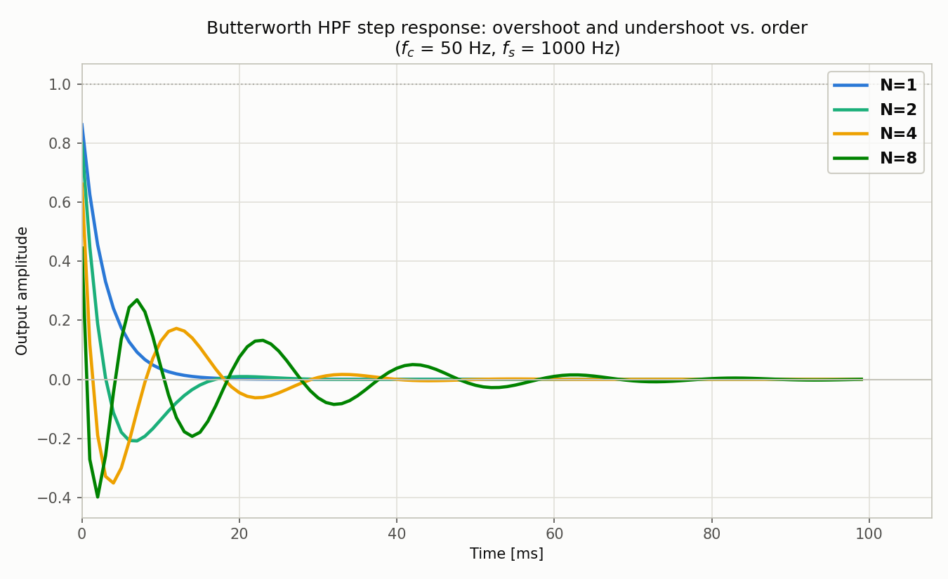
Practical implication: in applications where the input may contain step-like transients — a sudden change in sensor orientation, an electrode contact glitch — such as accelerometer gravity-component removal or ECG baseline correction, higher-order filters will produce more pronounced spurious overshoot/undershoot artifacts in the measured waveform, risking misdiagnosis or false detections. Choosing the filter order is a trade-off between roll-off steepness and tolerable ringing.
Differentiator-Like Behavior Near Cutoff and Noise Amplification
Consider the 1st-order highpass transfer function \((3)\) in the limit \(\omega \ll \omega_c\) :
\[ H_{HP}(j\omega) = \frac{j\omega}{j\omega + \omega_c} \approx \frac{j\omega}{\omega_c} \quad (\omega \ll \omega_c) \]This matches an ideal differentiator \(j\omega\) scaled by \(1/\omega_c\) : the magnitude is proportional to frequency (\(\lvert H_{HP}(j\omega)\rvert \approx \omega/\omega_c\) ), and the phase is a constant \(+90°\) lead. We verified the accuracy of this approximation numerically (\(f_c=100\) Hz):
import numpy as np

wc = 2 * np.pi * 100.0
test_f = np.array([1.0, 5.0, 10.0, 20.0])
w = 2 * np.pi * test_f
H_exact = (1j * w) / (1j * w + wc)
H_approx = (1j * w) / wc
for f, he, ha in zip(test_f, H_exact, H_approx):
    err = abs(abs(he) - abs(ha)) / abs(he) * 100
    print(f"f={f:5.1f}Hz  |H_exact|={abs(he):.5f}  |H_approx|={abs(ha):.5f}  error={err:.3f}%")
Results: the relative error is 0.005% at \(f=1\) Hz, 0.125% at \(f=5\) Hz, 0.499% at \(f=10\) Hz, and still only 1.980% at \(f=20\) Hz (one-fifth of \(f_c\) ) — confirming the approximation holds very well within a few tenths of the cutoff. More generally, an \(N\) th-order Butterworth highpass filter obeys the low-frequency asymptotic law \(\lvert H_{HP}(j\omega)\rvert \approx (\omega/\omega_c)^N\) for \(\omega \ll \omega_c\) (corresponding to a -20N dB/decade roll-off); numerically checking this across orders confirms the ratio to the theoretical value converges to within 0.87–0.97.
A differentiator emphasizes the rate of change of a signal — but this equally emphasizes measurement noise. We measured the actual change in SNR after applying a highpass filter to a low-frequency signal contaminated with noise:
import numpy as np
from scipy import signal

np.random.seed(42)
fs = 1000.0
t = np.arange(0, 2.0, 1 / fs)

clean = np.sin(2 * np.pi * 1.0 * t)          # Target signal (slow 1 Hz variation)
noise = 0.05 * np.random.randn(len(t))        # Broadband noise

fc_diff = 50.0  # Cutoff well above the signal band -> used as a differentiator
b, a = signal.butter(1, fc_diff / (fs / 2), btype='high')

skip = 500  # Discard the transient
clean_f = signal.lfilter(b, a, clean)[skip:]
noise_f = signal.lfilter(b, a, noise)[skip:]

snr_in = np.var(clean[skip:]) / np.var(noise[skip:])
snr_out = np.var(clean_f) / np.var(noise_f)
print(f"SNR_in  = {10*np.log10(snr_in):.2f} dB")
print(f"SNR_out = {10*np.log10(snr_out):.2f} dB")
print(f"Degradation = {10*np.log10(snr_in) - 10*np.log10(snr_out):.2f} dB")
print(f"Signal amplitude ratio std(clean_f)/std(clean) = {np.std(clean_f)/np.std(clean[skip:]):.5f}"
      f" (theoretical gain @1Hz = {abs((1j*2*np.pi*1.0)/(1j*2*np.pi*1.0+2*np.pi*fc_diff)):.5f})")
print(f"Noise amplitude ratio std(noise_f)/std(noise) = {np.std(noise_f)/np.std(noise[skip:]):.5f}")
Results:
- SNR (in): 22.68 dB → SNR (out): -10.34 dB (degradation of about 33 dB)
- Signal amplitude ratio: 0.02079 (matches the theoretical gain of 0.02000)
- Noise amplitude ratio: 0.93057
Because the target signal (1 Hz) is far below the cutoff (50 Hz), it is heavily attenuated to roughly 1/50 as theory predicts, while the broadband noise — with components at and above the cutoff — passes through almost unattenuated. Noise therefore becomes relatively dominant. This is the mechanism behind the well-known claim that “highpass filters used as differentiators amplify noise” (more precisely: noise becomes relatively more prominent than the signal; the filter’s gain itself never exceeds 1). Note also that using filtfilt (forward-backward, zero-phase filtering) squares the magnitude gain, so under identical conditions the SNR degradation grows to roughly 67 dB — we confirmed this as well. When differentiation (rate-of-change estimation) under noise is genuinely required in practice, a standalone highpass filter is usually insufficient; consider combining it with smoothing (e.g., a Savitzky-Golay derivative filter, or a bandpass-like design with an added lowpass stage).
Simple RC-Type Highpass Filters vs. Higher-Order Designs
The 1st-order highpass filter in equations \((3)\) /\((5)\) corresponds, in analog circuitry, to the simplest possible “DC-blocking filter” — a single resistor and capacitor (\(\omega_c = 1/RC\) ). For applications like microphone DC-bias removal or audio AC coupling, where phase behavior and ringing don’t matter and the only goal is to reject DC, this 1st-order RC design is entirely sufficient. It is simple to implement, its phase delay is gradual and monotonic, and — as shown above — it produces no undershoot at all.
By contrast, applications like ECG baseline-wander removal or vibration analysis — where the signal band and noise band are close together and a steep transition is required — typically use 4th- to 8th-order Butterworth or Chebyshev designs. But as shown above, higher order comes with increasing ringing (overshoot/undershoot) in response to step-like transients, so the choice of order is fundamentally a trade-off between transition-band steepness and time-domain waveform distortion. When phase distortion is a concern, consider this article’s filtfilt (zero-phase filtering), or pairing with a Bessel filter (maximally flat group delay), covered in a related article.
Python Implementation
IIR Highpass Filter with scipy.signal
import numpy as np
import matplotlib.pyplot as plt
from scipy import signal

# --- Parameters ---
fs = 1000.0      # Sampling frequency [Hz]
fc = 100.0       # Cutoff frequency [Hz]
order = 4        # Filter order

# --- Design Butterworth highpass filter ---
nyq = fs / 2.0   # Nyquist frequency
wn = fc / nyq    # Normalized cutoff frequency

b, a = signal.butter(order, wn, btype='high')

# --- Compute frequency response ---
w, h = signal.freqz(b, a, worN=8000, fs=fs)

# --- Plot ---
fig, (ax1, ax2) = plt.subplots(2, 1, figsize=(10, 8))

# Gain (dB)
ax1.semilogx(w, 20 * np.log10(np.abs(h) + 1e-10))
ax1.axvline(fc, color='r', linestyle='--', label=f'$f_c$ = {fc} Hz')
ax1.axhline(-3, color='gray', linestyle=':', label='-3 dB')
ax1.set_xlabel('Frequency [Hz]')
ax1.set_ylabel('Gain [dB]')
ax1.set_title(f'Butterworth Highpass Filter (order={order})')
ax1.legend()
ax1.grid(True, which='both', alpha=0.3)
ax1.set_xlim([1, nyq])
ax1.set_ylim([-80, 5])

# Phase
ax2.semilogx(w, np.angle(h, deg=True))
ax2.axvline(fc, color='r', linestyle='--')
ax2.set_xlabel('Frequency [Hz]')
ax2.set_ylabel('Phase [degrees]')
ax2.set_title('Phase Response')
ax2.grid(True, which='both', alpha=0.3)
ax2.set_xlim([1, nyq])

plt.tight_layout()
plt.savefig('highpass_response.png', dpi=150, bbox_inches='tight')
plt.show()
FIR Highpass Filter Design
IIR filters have nonlinear phase, but FIR filters can achieve linear phase. This is important in audio and medical signal processing where phase distortion is unacceptable.
from scipy.signal import firwin, freqz

# --- FIR highpass filter ---
numtaps = 101    # Number of taps (odd number recommended)
fir_hpf = firwin(
    numtaps,
    fc,
    pass_zero=False,  # Highpass specification
    fs=fs,
    window='hamming'
)

w_fir, h_fir = freqz(fir_hpf, worN=8000, fs=fs)

# IIR vs FIR comparison
plt.figure(figsize=(10, 5))
plt.semilogx(w, 20 * np.log10(np.abs(h) + 1e-10),
             label='IIR Butterworth (order=4)', linewidth=2)
plt.semilogx(w_fir, 20 * np.log10(np.abs(h_fir) + 1e-10),
             label=f'FIR Hamming (taps={numtaps})', linewidth=2, linestyle='--')
plt.axvline(fc, color='r', linestyle=':', alpha=0.7, label=f'$f_c$ = {fc} Hz')
plt.axhline(-3, color='gray', linestyle=':', alpha=0.7)
plt.xlabel('Frequency [Hz]')
plt.ylabel('Gain [dB]')
plt.title('Highpass Filter Comparison: IIR vs FIR')
plt.legend()
plt.grid(True, which='both', alpha=0.3)
plt.xlim([1, nyq])
plt.ylim([-80, 5])
plt.tight_layout()
plt.show()
Applying the Filter to a Signal
# --- Generate test signal ---
t = np.linspace(0, 1.0, int(fs), endpoint=False)

# Target signal: 200 Hz sine wave (high-frequency component)
signal_pure = np.sin(2 * np.pi * 200 * t)

# Noise: 5 Hz low-frequency drift (large amplitude) + white noise
noise = (
    2.0 * np.sin(2 * np.pi * 5 * t) +   # Low-frequency drift
    0.3 * np.random.randn(len(t))         # White noise
)

x_noisy = signal_pure + noise

# --- Apply filter ---
# lfilter: causal filter (real-time, has phase delay)
y_lfilter = signal.lfilter(b, a, x_noisy)

# filtfilt: zero-phase filter (offline, no phase delay)
y_filtfilt = signal.filtfilt(b, a, x_noisy)

# --- Comparison plot ---
fig, axes = plt.subplots(3, 1, figsize=(12, 8), sharex=True)

axes[0].plot(t[:300], x_noisy[:300], alpha=0.8, label='Noisy signal (with low-freq drift)')
axes[0].set_ylabel('Amplitude')
axes[0].set_title('Input Signal (with low-frequency drift)')
axes[0].legend()
axes[0].grid(True, alpha=0.3)

axes[1].plot(t[:300], y_lfilter[:300], color='orange', label='lfilter (causal)')
axes[1].plot(t[:300], signal_pure[:300], color='gray', linestyle='--', alpha=0.6, label='True signal')
axes[1].set_ylabel('Amplitude')
axes[1].set_title('After lfilter (with phase delay)')
axes[1].legend()
axes[1].grid(True, alpha=0.3)

axes[2].plot(t[:300], y_filtfilt[:300], color='green', label='filtfilt (zero-phase)')
axes[2].plot(t[:300], signal_pure[:300], color='gray', linestyle='--', alpha=0.6, label='True signal')
axes[2].set_ylabel('Amplitude')
axes[2].set_xlabel('Time [s]')
axes[2].set_title('After filtfilt (zero-phase)')
axes[2].legend()
axes[2].grid(True, alpha=0.3)

plt.tight_layout()
plt.savefig('highpass_filtering_result.png', dpi=150, bbox_inches='tight')
plt.show()
IIR vs FIR Design Comparison
| Property | IIR (Butterworth, etc.) | FIR |
|---|---|---|
| Phase response | Nonlinear (phase distortion) | Linear phase achievable |
| Number of coefficients | Small (\(2N+1\) approx.) | Large (tens to hundreds) |
| Computational cost | Low | High (depends on tap count) |
| Stability | Risk with high orders | Always stable |
| Stopband roll-off | Steep at low order | Improves with tap count |
| Group delay | Non-constant | Constant (\((N-1)/2\) samples) |
| Typical use | Real-time processing | Audio, medical signals |
Design guidelines:
- Low computational cost in real-time → IIR (Butterworth / Chebyshev)
- Linear phase required (audio, medical) → FIR (Hamming / Kaiser window)
- Offline processing, zero phase delay →
filtfilt(works with both IIR and FIR)
Effect of Filter Order
fig, ax = plt.subplots(figsize=(10, 6))

for ord_n in [1, 2, 4, 8]:
    b_n, a_n = signal.butter(ord_n, wn, btype='high')
    w_n, h_n = signal.freqz(b_n, a_n, worN=8000, fs=fs)
    ax.semilogx(w_n, 20 * np.log10(np.abs(h_n) + 1e-10), label=f'order={ord_n}')

ax.axhline(-3, color='gray', linestyle=':', label='-3 dB')
ax.axvline(fc, color='r', linestyle='--', alpha=0.5, label=f'$f_c$ = {fc} Hz')
ax.set_xlabel('Frequency [Hz]')
ax.set_ylabel('Gain [dB]')
ax.set_title('Effect of Filter Order on Highpass Response')
ax.legend()
ax.grid(True, which='both', alpha=0.3)
ax.set_xlim([1, nyq])
ax.set_ylim([-80, 5])
plt.tight_layout()
plt.show()
Order 1 gives a gradual roll-off, while order 8 gives a steep cutoff. However, IIR filters become numerically unstable at very high orders — order ≤ 8 is a practical guideline.
Recent Research Trends: Highpass Filtering in Biosignal Processing and Image Forensics
The step-response ringing (overshoot/undershoot) demonstrated above has been an actively revisited topic in biosignal processing research.
In EEG event-related potential (ERP) analysis, a 2023 study (a bioRxiv preprint from June 2023, subsequently published in Psychophysiology, following up on earlier filter-optimization work) quantitatively showed that pushing the highpass cutoff too high produces spurious opposite-polarity peaks before and after genuine ERP peaks. The paper states explicitly that “high-pass filters are inverted, so these filters typically produce artifactual opposite-polarity peaks before and after a true peak,” and sets a threshold requiring spurious-peak amplitude to stay within 5% of the true peak, yielding component-specific recommended cutoffs (e.g., 0.9 Hz for N170, 0.5 Hz for MMN/N2pc, 0.2 Hz for P3/N400). It also gives a concrete example in which “extreme high-pass filtering can cause a true P600 effect to produce an artifactual N400-like effect” — directly illustrating, with real data, the risk we quantified above: that increasing filter order (or cutoff) increases undershoot and can distort interpretation. A separate 2023 study in Scientific Reports similarly found that the optimal cutoff depends strongly on task type (0.1 Hz for a Face task, 0.5 Hz for an Oddball task, 0.75 Hz for a Go/No-go task), reinforcing that highpass filter design in EEG research remains highly signal-dependent.
For ECG baseline-wander removal, a cutoff around 0.5–1 Hz remains standard, and using a bidirectional (zero-phase) filter such as filtfilt continues to be the standard guidance for avoiding phase distortion. Raising the cutoff improves drift removal but trades off against distortion of clinically important low-frequency content (e.g., the S-T segment) — an ongoing design consideration.
In image processing and image forensics, highpass-style emphasis of high-frequency content continues to be used for detecting synthetic (GAN- or diffusion-generated) images. A 2024 training-free image-forensics method showed that simple handcrafted filters can capture high-frequency artifacts characteristic of generated images, suggesting that frequency-domain high-frequency emphasis remains a useful cue for forgery detection. That said, the specific filter designs (order, cutoff) vary by method, so readers interested in the details should consult the individual papers directly.
Sources:
- Optimal Filters for ERP Research II: Recommended Settings for Seven Common ERP Components (PMC10312706)
- EEG is better left alone (PMC9911389, Scientific Reports 2023)
- Data-Independent Operator: A Training-Free Artifact Representation Extractor for Generalizable Deepfake Detection (arXiv:2403.06803)
Practical Applications
| Application | Typical \(f_c\) | Notes |
|---|---|---|
| DC removal (microphone) | 20–80 Hz | Prevents signal saturation from DC offset |
| Accelerometer drift removal | 0.1–1 Hz | Removes gravity component (static bias) |
| ECG baseline wander removal | 0.5–1 Hz | Removes respiratory low-frequency variation |
| Image edge enhancement | — | 2D HPF sharpens contours |
| Vibration analysis noise removal | 1–10 Hz | Removes DC bias and mains hum from machinery |
Related Articles
- Lowpass Filter Design: Moving Average, Butterworth, Chebyshev — The dual of highpass filter design.
- Butterworth Filter Design: Theory and Python Implementation — The Butterworth prototype used in highpass design.
- Bandpass Filter Design: Theory and Python Implementation — Combining highpass and lowpass into a band-pass filter.
- FIR vs IIR Filters: A Comprehensive Comparison — Design philosophy differences between FIR and IIR filters.
- Notch Filter Design and Python Implementation — Band-stop filter that removes specific frequencies.
- Frequency Characteristics of the Exponential Moving Average Filter — EMA as a 1st-order IIR lowpass filter derived via Z-transform.
- FFT: Theory and Python Implementation — FFT fundamentals for verifying filter effects in the frequency domain.
- Adaptive Filters (LMS/RLS): Theory and Python Implementation — Filters that automatically adapt their frequency response.
- Bessel Filter: Theory and Python Implementation — IIR design with maximally flat group delay; useful as the HPF prototype when phase distortion must be minimized.
- Chebyshev Filter Design: Theory and Python Implementation — Equiripple alternative that yields a sharper transition than Butterworth at the same order.
- Bode Plot: Theory and Python Implementation — Hub article that visualizes the low-frequency roll-off and the \(+90N^\circ\) phase rotation of HPFs on a unified plot.
- Filter Design Selection Guide: 3 axes and characteristic comparison — Use this hub to position the highpass filter against alternatives during selection.
References
- Proakis, J. G., & Manolakis, D. G. (2006). Digital Signal Processing: Principles, Algorithms, and Applications. Pearson.
- scipy.signal.butter — SciPy documentation
- scipy.signal.filtfilt — SciPy documentation
Related Tools
- DevToolBox - Free Developer Tools — 85+ tools including JSON formatter, regex tester
- CalcBox - Everyday Calculation Tools — 61+ tools including statistics and frequency conversion