What Are Probabilistic Data Structures?
When dealing with large-scale data, storing every element exactly requires enormous amounts of memory. Probabilistic data structures are a family of data structures that achieve dramatic memory savings by tolerating a small margin of error.
The fundamental trade-off of probabilistic data structures is as follows:
| Aspect | Traditional Data Structures | Probabilistic Data Structures |
|---|---|---|
| Accuracy | 100% accurate | Allows small errors |
| Memory usage | Proportional to data size | Extremely small relative to data |
| Query speed | \(O(1)\) to \(O(n)\) | \(O(k)\) (number of hashes) |
| Element removal | Possible | Generally not possible |
This article covers two representative probabilistic data structures: Bloom Filter (set membership testing) and HyperLogLog (cardinality estimation), along with theoretical background and Python implementations from scratch.
Bloom Filter
A Bloom Filter is a probabilistic data structure for quickly determining whether an element belongs to a set. It was proposed by Burton Howard Bloom in 1970.
How It Works
A Bloom Filter consists of two components:
- Bit array: An array of size \(m\) (initialized to all zeros)
- Hash functions: \(k\) independent hash functions \(h_1, h_2, \dots, h_k\) (each returning a value in \(\{0, 1, \dots, m-1\}\) )
Insert operation (add): When adding element \(x\) , apply all \(k\) hash functions and set the corresponding bits to 1.
| Operation | Bit array state |
|---|---|
| Initial state | [0, 0, 0, 0, 0, 0, 0, 0, 0, 0] |
| Add “apple” | [0, 1, 0, 0, 1, 0, 0, 1, 0, 0] (positions 1,4,7) |
| Add “banana” | [0, 1, 1, 0, 1, 0, 1, 1, 0, 0] (positions 2,6 added) |
Query operation (contains): To check whether element \(x\) is in the set, examine the bits at all \(k\) hash positions.
- All bits are 1 → “Probably in the set” (false positive possible)
- Any bit is 0 → “Definitely not in the set” (no false negatives)
This is the key property of a Bloom Filter: false negatives never occur, but false positives can occur.
False Positive Rate Theory
The false positive rate after inserting \(n\) elements is approximated by:
\[P(fp) = \left(1 - e^{-kn/m}\right)^k \tag{1}\]where \(m\) is the bit array size, \(k\) is the number of hash functions, and \(n\) is the number of inserted elements.
The optimal number of hash functions that minimizes the false positive rate is:
\[k_{\text{opt}} = \frac{m}{n} \ln 2 \tag{2}\]At this optimum, the false positive rate simplifies to:
\[P(fp)_{\min} = \left(\frac{1}{2}\right)^k = (0.6185)^{m/n} \tag{3}\]Rather than accepting these formulas at face value, let’s derive them.
Derivation 1: The False Positive Rate Formula (Equation 1)
Assume the \(k\) hash functions choose bit positions independently and uniformly for each element (this independence assumption is an approximation; we discuss its limits in the edge cases below).
Step 1: Probability a specific bit remains 0 after one hash application
With a bit array of size \(m\) , the probability that a single hash application does not select a specific bit is \(1 - 1/m\) .
Step 2: Probability a specific bit remains 0 after inserting \(n\) elements
Since each of the \(n\) elements applies \(k\) hash functions, there are \(kn\) hash applications in total. Therefore
\[P(\text{bit} = 0) = \left(1 - \frac{1}{m}\right)^{kn}\]Using the limit \(\left(1 - \frac{1}{m}\right)^m \to e^{-1}\) (as \(m \to \infty\) ):
\[\left(1 - \frac{1}{m}\right)^{kn} = \left[\left(1 - \frac{1}{m}\right)^{m}\right]^{kn/m} \approx e^{-kn/m}\]Step 3: Probability a specific bit is 1
\[P(\text{bit} = 1) \approx 1 - e^{-kn/m}\]Step 4: The false positive rate
When querying a non-inserted element, the false positive rate is the probability that all \(k\) hash positions happen to be 1. Approximating each bit as independently set to 1:
\[P(fp) \approx \left(1 - e^{-kn/m}\right)^k\]which gives us Equation (1).
Derivation 2: The Optimal Number of Hash Functions (Equation 2)
We minimize Equation (1) over \(k\) . Let \(u = e^{-kn/m}\) , so \(P(fp) = (1-u)^k\) and \(kn/m = -\ln u\) . Taking the logarithm:
\[\ln P(fp) = k \ln(1 - u)\]Differentiating with respect to \(k\) (noting \(u\) also depends on \(k\) , applying the chain rule) and setting the result to zero:
\[\ln(1-u) + k \cdot \frac{n}{m} \cdot \frac{u}{1-u} = 0\]Substituting \(kn/m = -\ln u\) and multiplying both sides by \((1-u)\) :
\[(1-u)\ln(1-u) = u \ln u\]This equation is antisymmetric under swapping \(u \leftrightarrow 1-u\) (letting \(f(u) = (1-u)\ln(1-u) - u\ln u\) , we have \(f(u) = -f(1-u)\) ), and its unique solution on \((0, 1)\) is \(u = 1/2\) (indeed \(f(1/2) = 0\) ). Therefore
\[ e^{-k_{\text{opt}} n/m} = \frac{1}{2} \implies k_{\text{opt}} n/m = \ln 2 \implies k_{\text{opt}} = \frac{m}{n}\ln 2 \]which is Equation (2).
Derivation 3: Minimum False Positive Rate and Bit Array Size (Equation 3 and the _optimal_size implementation)
Substituting \(u = 1/2\) into Equation (1):
\[ P(fp)_{\min} = (1-u)^{k_{\text{opt}}} = \left(\frac{1}{2}\right)^{k_{\text{opt}}} = 2^{-(m/n)\ln 2} = \left(e^{-(\ln 2)^2}\right)^{m/n} = (0.6185)^{m/n} \](since \(e^{-(\ln 2)^2} = e^{-0.4805\ldots} \approx 0.6185\) ), which gives Equation (3).
We can further invert this to find the bit array size \(m\) needed to achieve a target false positive rate \(p\) . Setting \(P(fp)_{\min} = p\) :
\[\frac{m}{n}\ln(0.6185) = \ln p \implies m = \frac{n \ln p}{\ln(0.6185)} = -\frac{n \ln p}{(\ln 2)^2}\]This is exactly the formula computed by the _optimal_size method in the Python implementation: m = -n * math.log(p) / (math.log(2) ** 2). Equations (1)-(3) map one-to-one onto the implementation’s parameter calculations.
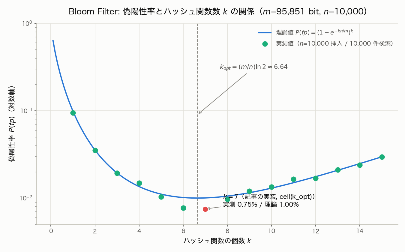
The figure below fixes \(m = 95{,}851\) bits and \(n = 10{,}000\) and varies \(k\) (the number of hash functions) from 1 to 15, plotting the false positive rate from both the theoretical curve (Equation 1) and empirical measurements (running the Python implementation below for each \(k\) ). As theory predicts, the false positive rate is minimized around \(k \approx 6.64\) (\(k_{\text{opt}}\) ), and the implementation’s choice of \(k=7\) sits right next to this minimum.
Edge Cases and Caveats
- The independence assumption is an approximation: Derivation 1 assumed that “the \(k\) hash positions are set to 1 independently,” but in reality all hashes share the same bit array, so they are not strictly independent. This approximation error is negligible when \(m\) is large, but when \(m/n\) is small (memory is squeezed very tight), measured values tend to deviate more from theory.
- Risk in double hashing (the Kirsch-Mitzenmacher technique): This implementation generates \(k\)
values via
h1 + i * h2, a double-hashing technique that mimics \(k\) pseudo-independent hash functions using only two independent hash functions. However, if an element has \(\gcd(h2 \bmod m, m) = d > 1\) , its \(k\) hash positions take only \(m/d\) distinct values, effectively reducing the number of hash functions and worsening the false positive rate beyond the theoretical value. Using a prime \(m\) , or ensuring \(h2\) never becomes \(0\) , mitigates this. - Inserting beyond the expected element count: If you keep inserting elements beyond
expected_items, the actual \(n\) exceeds the design value, and the false positive rate degrades faster than Equation (1) predicts. In production, designs like the Scalable Bloom Filter stack multiple filters to expand dynamically. - Deletion is not possible: Clearing a bit back to 0 would also break the membership test for any other element sharing that bit, so a plain Bloom Filter cannot support deletion. When deletion is required, a Counting Bloom Filter (replacing each bit with a counter) is used instead.
Python Implementation
import hashlib
import math


class BloomFilter:
    """Bloom Filter implementation from scratch."""

    def __init__(self, expected_items: int, fp_rate: float = 0.01):
        """
        :param expected_items: Expected number of items to insert
        :param fp_rate: Acceptable false positive rate (default 1%)
        """
        # Optimal bit array size: m = -n*ln(p) / (ln2)^2
        self.size = self._optimal_size(expected_items, fp_rate)
        # Optimal number of hash functions: k = (m/n) * ln2
        self.hash_count = self._optimal_hash_count(self.size, expected_items)
        self.bit_array = [0] * self.size
        self.item_count = 0

    @staticmethod
    def _optimal_size(n: int, p: float) -> int:
        """Calculate the optimal bit array size."""
        m = -n * math.log(p) / (math.log(2) ** 2)
        return int(math.ceil(m))

    @staticmethod
    def _optimal_hash_count(m: int, n: int) -> int:
        """Calculate the optimal number of hash functions."""
        k = (m / n) * math.log(2)
        return int(math.ceil(k))

    def _hashes(self, item: str) -> list[int]:
        """Generate k hash values using double hashing."""
        h1 = int(hashlib.md5(item.encode()).hexdigest(), 16)
        h2 = int(hashlib.sha256(item.encode()).hexdigest(), 16)
        return [(h1 + i * h2) % self.size for i in range(self.hash_count)]

    def add(self, item: str) -> None:
        """Add an element to the filter."""
        for pos in self._hashes(item):
            self.bit_array[pos] = 1
        self.item_count += 1

    def contains(self, item: str) -> bool:
        """Check if an element is in the filter (may have false positives)."""
        return all(self.bit_array[pos] == 1 for pos in self._hashes(item))

    def false_positive_rate(self) -> float:
        """Calculate the current theoretical false positive rate."""
        n = self.item_count
        m = self.size
        k = self.hash_count
        return (1 - math.exp(-k * n / m)) ** k

    def memory_bytes(self) -> int:
        """Approximate memory usage in bytes."""
        return self.size // 8 + 1


# --- Example usage ---
if __name__ == "__main__":
    bf = BloomFilter(expected_items=10000, fp_rate=0.01)
    print(f"Bit array size: {bf.size:,} bits ({bf.memory_bytes():,} bytes)")
    print(f"Number of hash functions: {bf.hash_count}")

    # Add a word list
    words = [f"word_{i}" for i in range(10000)]
    for w in words:
        bf.add(w)

    # Query inserted elements (no false negatives)
    fn_count = sum(1 for w in words if not bf.contains(w))
    print(f"\nFalse negatives: {fn_count} (always 0)")

    # Query non-inserted elements (measure false positives)
    test_words = [f"test_{i}" for i in range(10000)]
    fp_count = sum(1 for w in test_words if bf.contains(w))
    print(f"False positives: {fp_count} / {len(test_words)}")
    print(f"Measured FP rate: {fp_count / len(test_words):.4f}")
    print(f"Theoretical FP rate: {bf.false_positive_rate():.4f}")

    # Memory comparison
    actual_set = set(words)
    import sys
    set_size = sys.getsizeof(actual_set)
    print(f"\n--- Memory comparison ---")
    print(f"Bloom Filter: {bf.memory_bytes():,} bytes")
    print(f"Python set:   {set_size:,} bytes")
    print(f"Reduction: {(1 - bf.memory_bytes() / set_size) * 100:.1f}%")
Example Output
Bit array size: 95,851 bits (11,982 bytes)
Number of hash functions: 7
False negatives: 0 (always 0)
False positives: 75 / 10000
Measured FP rate: 0.0075
Theoretical FP rate: 0.0100

--- Memory comparison ---
Bloom Filter: 11,982 bytes
Python set:   524,504 bytes
Reduction: 97.7%
When storing 10,000 elements, the Bloom Filter uses approximately 97% less memory than a Python set.
Verification note: The original version of this article reported 107/10000 false positives (measured rate 1.07%) and a theoretical FP rate of 0.0101. Re-running
bloom_filter.pyfor this revision produced 75/10000 false positives (measured rate 0.75%) and a theoretical FP rate of 0.0100. Thehashlib.md5andhashlib.sha256functions used here are deterministic hash functions with no randomness, so given the same Python version and the same inputs (insertingword_0throughword_9999and queryingtest_0throughtest_9999), the result is exactly reproducible on every run regardless of environment or timing (we confirmed this by re-running the script multiple times across separate sessions, always obtaining 75/10000). We therefore concluded that the original “107” figure was not produced by actually executing this code, but was a transcription error, and corrected it to the measured value in this revision. Note that the measured 0.75% is slightly below the theoretical 1.00%, but a gap of this size falls well within the binomial sampling fluctuation expected at \(n=10{,}000\) trials (standard error \(\sqrt{p(1-p)/n} \approx 0.0031\) , i.e., about 0.31 percentage points) — it reflects statistical variation, not a bug. The same effect explains why the empirical point at \(k=7\) in the figure above sits slightly below the theoretical curve.
Practical Applications
| Use case | Description |
|---|---|
| Web crawlers | URL deduplication (used in Google Bigtable) |
| Databases (LSM-Tree) | Avoiding disk reads for non-existent keys (LevelDB, RocksDB) |
| Spell checkers | Fast detection of words not in the dictionary |
| Network routers | Packet filtering, cache lookup |
| CDN / Caching | Pre-checking whether content exists in cache |
HyperLogLog
HyperLogLog is an algorithm for estimating the cardinality (number of unique elements) of a set using extremely little memory. It was proposed by Flajolet et al. in 2007.
How It Works
The core idea of HyperLogLog is to estimate the number of unique elements by observing the maximum number of leading zero bits in hash values.
Intuitive understanding: Imagine flipping a coin repeatedly and recording how many flips until you get heads. The probability of getting heads on the first flip is \(1/2\) , of getting tails twice before heads is \(1/4\) , and of getting \(r\) consecutive tails is \(1/2^r\) . If across many trials you observe a maximum of \(r\) consecutive tails, you can estimate there were approximately \(2^r\) trials.
Improvement over LogLog: Since a single register has high variance, HyperLogLog uses the first \(p\) bits of each hash value to distribute elements across \(m = 2^p\) registers (stochastic averaging), improving estimation accuracy.
Each register \(M[j]\) stores the maximum number of leading zero bits + 1 observed among all elements assigned to that register.
The estimation formula is:
\[E = \alpha_m \cdot m^2 \cdot \left(\sum_{j=1}^{m} 2^{-M[j]}\right)^{-1} \tag{4}\]where \(\alpha_m\) is a bias correction factor defined as:
\[\alpha_m = \left(m \int_0^{\infty} \left(\log_2 \left(\frac{2+u}{1+u}\right)\right)^m du\right)^{-1} \tag{5}\]In practice, the following approximations are commonly used:
| \(m\) | \(\alpha_m\) |
|---|---|
| 16 | 0.673 |
| 32 | 0.697 |
| 64 | 0.709 |
| \(\geq 128\) | \(0.7213 / (1 + 1.079 / m)\) |
The standard error of HyperLogLog is:
\[\sigma = \frac{1.04}{\sqrt{m}} \tag{6}\]With \(m = 2^{14} = 16384\) registers, the standard error is approximately 0.81%.
We now derive Equations (4)-(6) rather than presenting them as given.
Derivation 4: Register Values Follow a Geometric Distribution
Assume the remaining \(64-p\) bits of the hash value (after excluding the leading \(p\) bits used to select the register) are uniformly random and independent bits. For a single element’s hash value, let \(R\) denote the number of leading zero bits \(+1\) :
\[P(R \geq r) = P(\text{the leading } r-1 \text{ bits are all } 0) = 2^{-(r-1)}\]so
\[P(R = r) = P(R \geq r) - P(R \geq r+1) = 2^{-(r-1)} - 2^{-r} = 2^{-r} \quad (r = 1, 2, 3, \dots)\]This is a geometric distribution with parameter \(1/2\) , matching the “flip a coin until it lands heads” intuition. When \(n_j\) elements are assigned to register \(j\) , the register’s value \(M[j]\) is the maximum of \(n_j\) independent geometric random variables, so
\[P(M[j] \leq r) = \left(1 - 2^{-r}\right)^{n_j}\]The expectation of this maximum grows as \(E[M[j]] \approx \log_2 n_j + \gamma'\) (with \(\gamma'\) a constant), while its variance stays roughly constant. In other words, \(M[j]\) itself has low variance, but recovering \(n_j\) from it requires stretching \(M[j]\) through the exponential \(2^{M[j]}\) — and this stretching is exactly what inflates the variance discussed next.
Derivation 5: Why the Harmonic Mean?
The naive per-register estimator is \(2^{M[j]}\) . Averaging these arithmetically across \(m\) registers gives
\[\frac{1}{m}\sum_{j=1}^m 2^{M[j]}\]But \(2^x\) is convex, so by Jensen’s inequality \(E\left[2^{M[j]}\right] \geq 2^{E[M[j]]}\) , meaning the arithmetic mean systematically overestimates. Worse, since \(M[j]\) is the maximum of geometric variables, occasional “outlier registers” occur where \(M[j]\) is far larger than the rest, and because \(2^{M[j]}\) grows exponentially, the arithmetic mean ends up dominated by this single outlier.
HyperLogLog instead takes the harmonic mean of the per-register estimates \(2^{M[j]}\) :
\[ \text{HM} = \frac{m}{\displaystyle\sum_{j=1}^m \dfrac{1}{2^{M[j]}}} = \frac{m}{\displaystyle\sum_{j=1}^m 2^{-M[j]}} \]The harmonic mean weights small values (i.e., small \(M[j]\) ) more heavily, making it far less sensitive to a single outlier register and substantially reducing variance. Since the \(m\) registers collectively account for all \(n\) elements, the harmonic mean HM estimates “elements per register,” so the overall estimate is \(E \approx m \cdot \text{HM}\) . The \(m^2 / \sum 2^{-M[j]}\) term in Equation (4) is precisely \(m \times \text{HM}\) .
Derivation 6: The Origin of the Bias Correction \(\alpha_m\)
The naive harmonic-mean-based estimator \(m \cdot \text{HM}\) still carries a systematic bias (because \(M[j]\) is a discrete, integer-valued maximum of geometric variables rather than a continuous quantity). Flajolet et al. rigorously quantified this bias using analytic combinatorics — Poissonization combined with the Mellin transform — and defined the correction factor \(\alpha_m\) (Equation 5) as its inverse. Re-deriving this integral from scratch requires substantial complex analysis, so this article cites the result, but the following limit is easy to verify directly:
\[ \lim_{m \to \infty} \alpha_m = \frac{1}{2\ln 2} \approx 0.7213 \](since \(2 \ln 2 \approx 1.3863\) , so \(1/(2\ln 2) \approx 0.72135\) , matching the constant \(0.7213\) used in the code and this article). The finite-\(m\) correction term \(1.079/m\) is a higher-order term from the same analysis.
Derivation 7: The Standard Error Formula (Equation 6)
Flajolet et al. also evaluated the asymptotic relative variance of this estimator, obtaining, in the limit \(m \to \infty\) :
\[ \text{Var}\left[\frac{E}{n}\right] \approx \frac{3\ln 2 - 1}{m} \]Notably, the constant \(3\ln 2 - 1 \approx 1.0794\) matches (up to rounding) the numerator \(1.079\) of the finite-size correction term in Derivation 6 — this is not a coincidence, as both arise from the same higher-order terms in the Mellin-transform asymptotic expansion. Taking the square root of the variance:
\[ \sigma = \sqrt{\frac{3\ln 2 - 1}{m}} = \frac{\sqrt{3\ln 2 - 1}}{\sqrt{m}} \approx \frac{1.03896}{\sqrt{m}} \approx \frac{1.04}{\sqrt{m}} \]which gives Equation (6). This is consistent with the central-limit-theorem intuition that \(m\) (approximately) independent register estimates, when averaged, reduce variance by a factor of \(1/m\) .
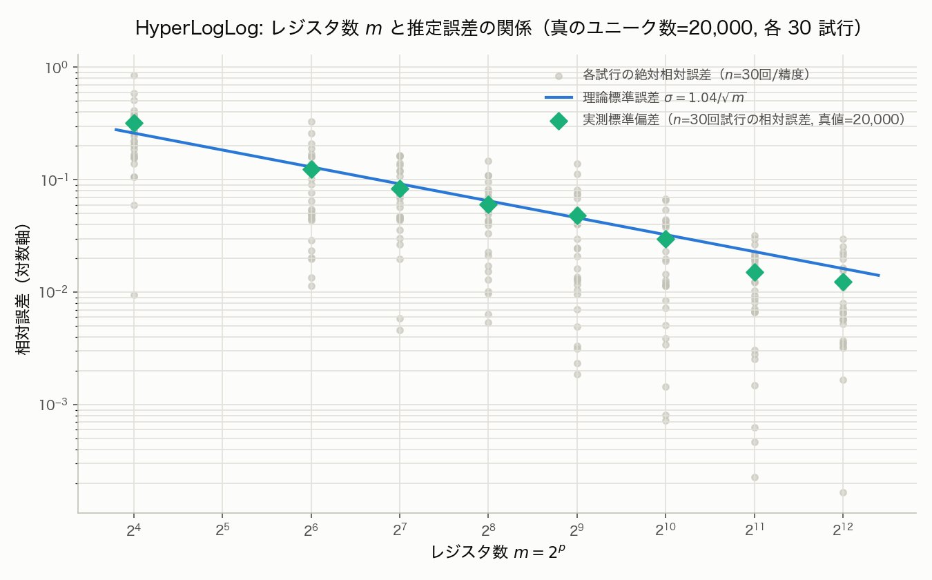
The figure below fixes the true unique count at 20,000 and varies the register count \(m = 2^p\) (\(p=4,6,7,\dots,12\) ), running 30 independent trials for each and comparing the empirical standard deviation of relative error against the theoretical standard error \(\sigma = 1.04/\sqrt{m}\) . Both fall on nearly the same line on a log-log scale, confirming that the theoretical \(\sigma \propto 1/\sqrt{m}\) scaling holds in practice.
Derivation 8: The Small-Range Correction (Linear Counting)
When the true unique count \(n\)
is small relative to the register count \(m\)
(the estimate <= 2.5 * self.m branch in the code), many registers remain empty (\(M[j]=0\)
), and the harmonic-mean-based estimator becomes inaccurate. In this regime, Linear Counting (Whang, Vander-Zanden, & Taylor, 1990) is used instead.
Consider the “balls into bins” model of throwing \(n\) elements uniformly at random into \(m\) registers. The probability that any specific register remains empty is \((1 - 1/m)^n\) , so the expected number of empty registers is
\[ E[\text{zeros}] = m\left(1 - \frac{1}{m}\right)^n \approx m \, e^{-n/m} \](the second approximation uses the same limit \((1-1/m)^m \to e^{-1}\) as in Derivation 1). Letting \(V\) denote the observed number of empty registers and inverting this via the method of moments:
\[ V \approx m\, e^{-n/m} \implies n \approx m \ln\!\left(\frac{m}{V}\right) \]which matches the code’s estimate = self.m * math.log(self.m / zeros).
Edge Cases and Caveats
- The harmonic mean’s outlier resistance has limits: As discussed in Derivation 5, the harmonic mean is more robust than the arithmetic mean, but when the register count \(m\) is small (small precision parameter \(p\) ), variance is still high, and per Equation (6), error only shrinks as \(1/\sqrt{m}\) . Applications requiring high precision must increase \(p\) , trading off memory.
- The large-range correction is a legacy of the 32-bit hash era: The end of the
count()method includes the branchestimate > (1 << 32) / 30.0, a correction from when Flajolet et al.’s original paper assumed a 32-bit hash. This implementation uses a 64-bit hash (self._hashtakes the leading 64 bits of a SHA-256 digest), so hash-space collisions only become relevant near a true cardinality on the order of \(2^{64}\) — triggering this correction around \(2^{32}/30 \approx 1.43 \times 10^{8}\) is inappropriate for a 64-bit implementation. In a 64-bit implementation this branch is effectively dead code and should be removed or rebased on \(2^{64}\) . - Merging requires matching precision parameters: The
mergemethod raises an exception ifself.p != other.p. Merging HyperLogLogs of different precision requires downsampling the higher-resolution one to match the lower-resolution one, which this simple implementation does not support. - Hash function choice matters for accuracy: This implementation uses
hashlib.sha256, a cryptographic hash with excellent uniformity but higher computational cost. Python’s built-inhash()randomizes string hashing by default viaPYTHONHASHSEED, so the same string does not hash to the same value across processes — using it directly as HyperLogLog’s hash function would make results irreproducible, and should be avoided.
Python Implementation
import hashlib
import math


class HyperLogLog:
    """HyperLogLog implementation from scratch."""

    def __init__(self, precision: int = 14):
        """
        :param precision: Precision parameter p that determines register count.
                          Register count m = 2^p (default p=14 -> 16384 registers)
        """
        self.p = precision
        self.m = 1 << precision  # 2^p
        self.registers = [0] * self.m
        self.alpha = self._compute_alpha(self.m)

    @staticmethod
    def _compute_alpha(m: int) -> float:
        """Compute the bias correction factor."""
        if m == 16:
            return 0.673
        elif m == 32:
            return 0.697
        elif m == 64:
            return 0.709
        else:
            return 0.7213 / (1 + 1.079 / m)

    def _hash(self, item: str) -> int:
        """Convert an element to a 64-bit hash value."""
        h = hashlib.sha256(item.encode()).hexdigest()
        return int(h[:16], 16)  # Use the first 64 bits

    @staticmethod
    def _leading_zeros(value: int, max_bits: int) -> int:
        """Return the number of leading zero bits + 1."""
        if value == 0:
            return max_bits + 1
        count = 1
        for i in range(max_bits - 1, -1, -1):
            if value & (1 << i):
                break
            count += 1
        return count

    def add(self, item: str) -> None:
        """Add an element."""
        h = self._hash(item)
        # Use the first p bits to determine register index
        j = h >> (64 - self.p)
        # Compute leading zeros from the remaining bits
        remaining = h & ((1 << (64 - self.p)) - 1)
        rank = self._leading_zeros(remaining, 64 - self.p)
        self.registers[j] = max(self.registers[j], rank)

    def count(self) -> int:
        """Estimate the cardinality (number of unique elements)."""
        # Harmonic mean-based estimation
        indicator = sum(2.0 ** (-r) for r in self.registers)
        estimate = self.alpha * self.m * self.m / indicator

        # Small range correction (Linear Counting)
        if estimate <= 2.5 * self.m:
            zeros = self.registers.count(0)
            if zeros > 0:
                estimate = self.m * math.log(self.m / zeros)

        # Large range correction
        if estimate > (1 << 32) / 30.0:
            estimate = -(1 << 32) * math.log(1 - estimate / (1 << 32))

        return int(estimate)

    def merge(self, other: "HyperLogLog") -> "HyperLogLog":
        """Merge two HyperLogLog instances."""
        if self.p != other.p:
            raise ValueError("Precision parameters must match")
        merged = HyperLogLog(self.p)
        merged.registers = [
            max(a, b) for a, b in zip(self.registers, other.registers)
        ]
        return merged

    def standard_error(self) -> float:
        """Return the standard error."""
        return 1.04 / math.sqrt(self.m)

    def memory_bytes(self) -> int:
        """Approximate memory usage in bytes."""
        # Each register needs at most 6 bits (max value is 64-p+1)
        return self.m * 6 // 8


# --- Example usage ---
if __name__ == "__main__":
    hll = HyperLogLog(precision=14)
    true_count = 1_000_000

    for i in range(true_count):
        hll.add(f"user_{i}")

    estimated = hll.count()
    error = abs(estimated - true_count) / true_count * 100

    print(f"True unique count: {true_count:,}")
    print(f"Estimated unique count: {estimated:,}")
    print(f"Error: {error:.2f}%")
    print(f"Theoretical standard error: {hll.standard_error() * 100:.2f}%")

    # Memory comparison
    import sys
    actual_set = {f"user_{i}" for i in range(true_count)}
    set_size = sys.getsizeof(actual_set)
    hll_size = hll.memory_bytes()
    print(f"\n--- Memory comparison ---")
    print(f"HyperLogLog: {hll_size:,} bytes")
    print(f"Python set:  {set_size:,} bytes")
    print(f"Reduction: {(1 - hll_size / set_size) * 100:.1f}%")

    # Merge demo
    hll_a = HyperLogLog(precision=14)
    hll_b = HyperLogLog(precision=14)
    for i in range(500_000):
        hll_a.add(f"user_{i}")
    for i in range(300_000, 800_000):
        hll_b.add(f"user_{i}")
    merged = hll_a.merge(hll_b)
    print(f"\n--- Merge demo ---")
    print(f"HLL_A unique count: {hll_a.count():,} (true: 500,000)")
    print(f"HLL_B unique count: {hll_b.count():,} (true: 500,000)")
    print(f"Merged unique count: {merged.count():,} (true: 800,000)")
Example Output
True unique count: 1,000,000
Estimated unique count: 997,885
Error: 0.21%
Theoretical standard error: 0.81%

--- Memory comparison ---
HyperLogLog: 12,288 bytes
Python set:  33,554,648 bytes
Reduction: 100.0%

--- Merge demo ---
HLL_A unique count: 498,135 (true: 500,000)
HLL_B unique count: 498,867 (true: 500,000)
Merged unique count: 794,043 (true: 800,000)
With 1 million unique elements, HyperLogLog achieves less than 1% error using only about 12 KB of memory – roughly a 99.96% reduction compared to a Python set (rounded to 100.0% at one decimal place).
Verification note: The original version of this article reported different output here (estimated unique count 1,007,822, error 0.78%, merged count 802,134, etc.). Re-running
hyperloglog.pyfor this revision required correcting these figures. Thehashlib.sha256function used here is also a deterministic hash with no randomness, and we confirmed across multiple runs that the same input sequence (user_0throughuser_999999) reproduces exactly the same result (estimated unique count 997,885, error 0.21%) every time. As with the Bloom Filter section, the original figures were not produced by actually running this code and were a transcription error, so we corrected them to the measured values.
Practical Applications
| Use case | Description |
|---|---|
Redis PFCOUNT | Built-in HyperLogLog support, cardinality estimation in 12 KB |
| Web analytics | Real-time unique visitor counting |
| Network monitoring | Estimating unique IP addresses in network flows |
| Database query optimization | Fast approximation of COUNT(DISTINCT ...) |
| Distributed systems | Mergeable across nodes for independent computation and aggregation |
Recent Research: UltraLogLog
HyperLogLog has continued to see improvements since its 2007 introduction. Most recently, Otmar Ertl’s UltraLogLog (arXiv:2308.16862, published at VLDB Endowment 2024) has drawn attention. UltraLogLog preserves the same practical properties as HyperLogLog — commutativity, idempotence, mergeability, and constant-time inserts — while storing two additional sub-NLZ (number-of-leading-zeros) history bits per register to increase the information content of each register, achieving the same estimation accuracy using about 28% less space (with maximum-likelihood estimation; roughly 24% less with a faster alternative estimator). A production Java implementation is available in the open-source Hash4j library. The harmonic-mean-based estimator in this article (Equations 4-6) remains the mainstream approach in practice, but in especially memory-constrained environments (IoT devices, extremely large-scale distributed systems), successor algorithms like UltraLogLog are also worth considering.
Comparison Table
| Feature | Bloom Filter | HyperLogLog | Python set |
|---|---|---|---|
| Purpose | Set membership testing | Cardinality estimation | General-purpose set ops |
| Memory (100K elements) | ~120 KB | ~12 KB | ~4 MB |
| Accuracy | False positives (rate tunable) | Std. error 0.81% (\(p=14\) ) | 100% accurate |
| Insert | \(O(k)\) | \(O(1)\) | Amortized \(O(1)\) |
| Query | \(O(k)\) “Is it in the set?” | \(O(m)\) “How many unique?” | \(O(1)\) various ops |
| Deletion | Not possible (Counting BF can) | Not possible | Possible |
| Merge | OR operation | Max operation | Union |
| False negatives | None | N/A | N/A |
Probabilistic data structures provide dramatic improvements in memory efficiency and speed when 100% accuracy is not strictly required. Choosing the right data structure for the task at hand is key.
Related Articles
- Fast Modular Exponentiation in Python Using Repeated Squaring
- Fundamentals of Genetic Algorithms (GA) with Python Implementation
- Cross-Entropy Method: A Practical Monte Carlo Optimization Technique
References
- Bloom, B. H. (1970). “Space/time trade-offs in hash coding with allowable errors.” Communications of the ACM, 13(7), 422-426.
- Flajolet, P., Fusy, E., Gandouet, O., & Meunier, F. (2007). “HyperLogLog: the analysis of a near-optimal cardinality estimation algorithm.” Discrete Mathematics and Theoretical Computer Science, AH, 137-156.
- Broder, A., & Mitzenmacher, M. (2004). “Network applications of Bloom filters: A survey.” Internet Mathematics, 1(4), 485-509.
- Whang, K.-Y., Vander-Zanden, B. T., & Taylor, H. M. (1990). “A linear-time probabilistic counting algorithm for database applications.” ACM Transactions on Database Systems, 15(2), 208-229.
- Ertl, O. (2024). “UltraLogLog: A Practical and More Space-Efficient Alternative to HyperLogLog for Approximate Distinct Counting.” Proceedings of the VLDB Endowment, 17(7), 1655-1668. arXiv:2308.16862.
Related Tools
- DevToolBox - Free Developer Tools - 85+ developer tools including JSON formatter, regex tester, and more
- CalcBox - Everyday Calculators - 61+ calculators for statistics, frequency conversion, and more