Introduction
The Chebyshev filter achieves a sharper transition band than a Butterworth filter of the same order by allowing equiripple in the passband (Type I) or stopband (Type II).
Where the Butterworth filter maximizes flatness in the passband, the Chebyshev filter trades that flatness for steeper rolloff. This article covers the mathematical foundations of both types and their practical design with SciPy.
Chebyshev Polynomials
Chebyshev filter frequency responses are based on the Chebyshev polynomial \(T_N(x)\) :
\[T_N(x) = \begin{cases} \cos(N \arccos x) & |x| \leq 1 \\ \cosh(N \operatorname{arccosh} x) & |x| > 1 \end{cases} \tag{1}\]The first few Chebyshev polynomials are:
| Order \(N\) | \(T_N(x)\) |
|---|---|
| 0 | \(1\) |
| 1 | \(x\) |
| 2 | \(2x^2 - 1\) |
| 3 | \(4x^3 - 3x\) |
| 4 | \(8x^4 - 8x^2 + 1\) |
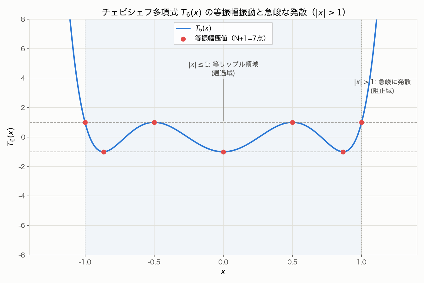
Within \(|x| \leq 1\) , the Chebyshev polynomial oscillates between \(-1\) and \(+1\) with equal amplitude — this property produces the equiripple characteristic in the filter.
Why the Chebyshev Polynomial Specifically: Minimax Optimality
The Chebyshev filter picks the Chebyshev polynomial as its equiripple building block for a reason deeper than “it oscillates.” Chebyshev himself proved the following theorem in 1854.
Chebyshev’s minimax theorem: among all monic (leading coefficient \(1\) ) polynomials of degree \(N\) on \([-1,1]\) , the one that minimizes the maximum absolute value (sup norm) is
\[ \tilde{T}_N(x) = \frac{1}{2^{N-1}} T_N(x) \]and the minimum value achieved is \(2^{1-N}\) .
Proof sketch (by contradiction): \(T_N(x) = \cos(N\arccos x)\) attains an alternating sequence of extrema at \(N+1\) points inside the interval (equioscillation). Write the extremal points and their values as
\[ x_m = \cos\!\left(\frac{m\pi}{N}\right), \qquad T_N(x_m) = (-1)^m \qquad (m=0,1,\ldots,N) \]Suppose a monic polynomial \(q(x)\) existed with a smaller sup norm than \(\tilde{T}_N\) . Define the difference
\[ \Delta(x) = \tilde{T}_N(x) - q(x) \]Since both are monic, the leading terms cancel and \(\Delta(x)\) has degree at most \(N-1\) . Because \(q\) ’s sup norm is assumed smaller than the extremal value (\(=1\) ), the sign of \(\Delta\) at the \(N+1\) points above must match the sign of \(T_N\) there, alternating \(N+1\) times. A continuous function whose sign alternates at \(N+1\) points must have at least \(N\) zeros inside the interval — but this exceeds the maximum number of zeros a degree-\((N-1)\) polynomial can have (\(N-1\) ), a contradiction. Hence \(\tilde{T}_N\) is the unique minimizer.
This theorem means that, under the constraint of staying within passband ripple \(R_p\) , no degree-\(N\) polynomial approximation other than the Chebyshev polynomial can achieve a sharper transition band. The Chebyshev filter is therefore the theoretically optimal choice among amplitude responses expressible as polynomials (allowing rational functions instead opens the door to the even sharper elliptic filter , which generalizes this single-period, polynomial theory to a double-period, rational-function theory via the Zolotarev rational function — see that article for details).
Numerical verification: we confirm the proof’s claim (any deviation from the monic Chebyshev polynomial increases the sup norm) directly. Take the monic Chebyshev polynomial of degree \(N=5\) ,
\[ \tilde{T}_5(x) = T_5(x)/2^4 \]and add a random lower-degree polynomial scaled by a small coefficient \(\varepsilon_p\) , then observe how the sup norm changes.
import numpy as np
from numpy.polynomial import chebyshev as C

N = 5
x = np.linspace(-1, 1, 400001)

coeffs = np.zeros(N + 1); coeffs[N] = 1.0
monic_cheb = C.chebval(x, coeffs) / 2**(N - 1)
sup_cheb = np.max(np.abs(monic_cheb))

rng = np.random.default_rng(1)
direction = rng.normal(size=N)
direction /= np.linalg.norm(direction)
powers = np.vstack([x**i for i in range(N)])

print(f"sup-norm of monic Chebyshev T_5/2^4 = {sup_cheb:.8f}  (theory 2^-4 = {2**(1-N):.8f})")
for eps_p in [0.0, 0.001, 0.005, 0.01, 0.05, -0.001, -0.01]:
    perturbed = monic_cheb + eps_p * (direction @ powers)
    sup_p = np.max(np.abs(perturbed))
    print(f"  eps={eps_p:+.4f}: sup-norm = {sup_p:.8f}  (delta {sup_p - sup_cheb:+.8f})")
Output:
sup-norm of monic Chebyshev T_5/2^4 = 0.06250000  (theory 2^-4 = 0.06250000)
  eps=+0.0000: sup-norm = 0.06250000  (delta +0.00000000)
  eps=+0.0010: sup-norm = 0.06309459  (delta +0.00059459)
  eps=+0.0050: sup-norm = 0.06547294  (delta +0.00297294)
  eps=+0.0100: sup-norm = 0.06844589  (delta +0.00594589)
  eps=+0.0500: sup-norm = 0.09222943  (delta +0.02972943)
  eps=-0.0010: sup-norm = 0.06361524  (delta +0.00111524)
  eps=-0.0100: sup-norm = 0.07365243  (delta +0.01115243)
For every random perturbation direction and sign tested, the sup norm strictly increases (delta is always positive), confirming numerically that \(\varepsilon_p=0\) (the Chebyshev polynomial itself) is a local minimum.
The figure below shows the \(N=6\) Chebyshev polynomial \(T_6(x)\) and its \(N+1=7\) equioscillation extrema: bounded oscillation between \(\pm 1\) for \(|x|\leq 1\) , and rapid divergence for \(|x|>1\) .
Chebyshev Type I Filter
Magnitude Response
The magnitude squared function of an \(N\) -th order Chebyshev Type I lowpass filter is:
\[|H(j\Omega)|^2 = \frac{1}{1 + \varepsilon^2 T_N^2\!\left(\dfrac{\Omega}{\Omega_p}\right)} \tag{2}\]where:
- \(\varepsilon\) : ripple factor (\(\varepsilon > 0\) )
- \(\Omega_p\) : passband edge angular frequency
- \(T_N\) : Chebyshev polynomial of order \(N\)
In the passband (\(\Omega \leq \Omega_p\) ),
\[ T_N(\Omega/\Omega_p) \in [-1, 1] \]so the magnitude ripples between \(1/\sqrt{1+\varepsilon^2}\) and \(1\) with equal amplitude. The relationship between passband ripple \(R_p\) [dB] and the ripple factor is:
\[\varepsilon = \sqrt{10^{R_p/10} - 1} \tag{3}\]Edge Case: DC Gain Depends on Order Parity
Substituting \(\Omega=0\) into equation (2), the DC gain is determined entirely by \(T_N(0)=\cos(N\arccos 0)=\cos(N\pi/2)\) :
- Odd \(N\) : \(N\pi/2\) is an odd multiple of \(\pi/2\) , so \(\cos(N\pi/2)=0\) and \(|H(j0)|^2=1\) (DC gain is exactly 0 dB, full passband)
- Even \(N\) : \(\cos(N\pi/2)=\pm 1\) , so \(|H(j0)|^2=1/(1+\varepsilon^2)\) (DC gain equals the passband ripple floor, \(-R_p\) dB)
This is an easy pitfall for beginners: it’s tempting to assume “the passband ripples around 0 dB” and expect 0 dB at DC regardless of order, but for even orders the DC gain itself starts at \(-R_p\) dB. Let’s verify numerically.
import numpy as np
from scipy import signal

fs = 100_000
fp = 100
rp = 1.0
eps = np.sqrt(10**(rp / 10) - 1)

print(f"{'N':<4}{'T_N(0)':>10}{'theory DC[dB]':>16}{'measured DC[dB]':>18}")
for N in [3, 4, 5, 6, 7, 8]:
    TN0 = np.cos(N * np.pi / 2)
    H2 = 1 / (1 + eps**2 * TN0**2)
    gain_theory_db = 10 * np.log10(H2)

    sos = signal.cheby1(N, rp, fp, btype='low', fs=fs, output='sos')
    _, h = signal.sosfreqz(sos, worN=[1e-6], fs=fs)
    gain_meas_db = 20 * np.log10(np.abs(h[0]))

    print(f"{N:<4}{TN0:>10.3f}{gain_theory_db:>16.4f}{gain_meas_db:>18.4f}")
Output:
N       T_N(0)  theory DC[dB]  measured DC[dB]
3       -0.000            0.0000            0.0000
4        1.000           -1.0000           -1.0000
5        0.000            0.0000           -0.0000
6       -1.000           -1.0000           -1.0000
7       -0.000            0.0000            0.0000
8        1.000           -1.0000           -1.0000
Theory and the scipy.signal.cheby1 measurement agree exactly: odd orders (\(N=3,5,7\)
) give a DC gain of exactly 0 dB, while even orders (\(N=4,6,8\)
) give exactly \(-R_p=-1\)
dB. This parity dependence is unique to Chebyshev Type I — Butterworth (equation 1) always has \(|H|=1\)
at \(\Omega=0\)
regardless of order. Applications requiring an exact 0 dB DC pass (e.g. DC-coupled instrumentation amplifier stages) need to account for this offset when choosing an even order.
Pole Locations
The poles of a Chebyshev Type I filter lie on an ellipse. For \(k = 1, 2, \ldots, N\) :
\[\sigma_k = -\sinh\!\left(\frac{\operatorname{arcsinh}(1/\varepsilon)}{N}\right)\sin\theta_k \tag{4}\]\[\omega_k = \cosh\!\left(\frac{\operatorname{arcsinh}(1/\varepsilon)}{N}\right)\cos\theta_k \tag{5}\]where \(\theta_k = \dfrac{\pi(2k-1)}{2N}\) . Only the left half-plane poles
\[ s_k = \sigma_k + j\omega_k \]are used for stability.
Deriving equations (4) and (5)
We seek the values of \(s\) (the poles) that zero the denominator of the normalized (\(\Omega_p=1\) ) magnitude-squared function. The denominator of \(H(s)H(-s)\) becomes \(1+\varepsilon^2 T_N^2(-js)\) via the analytic continuation \(\Omega \to -js\) , so the poles solve
\[ T_N(-js) = \pm \frac{j}{\varepsilon} \]Substitute \(-js = \cos\theta\) with \(\theta = u+jv\) (\(u,v\) real). Since the identity \(T_N(\cos\theta)=\cos(N\theta)\) continues to hold for complex \(\theta\) ,
\[ \cos(Nu+jNv) = \cos(Nu)\cosh(Nv) - j\sin(Nu)\sinh(Nv) = \pm\frac{j}{\varepsilon} \]The right side is purely imaginary, so the real part must vanish. Since \(\cosh(Nv) > 0\) always,
\[ \cos(Nu) = 0 \ \Longrightarrow\ u_k = \theta_k = \frac{(2k-1)\pi}{2N} \qquad (k=1,\ldots,N) \]giving \(N\) solutions for \(\theta_k \in (0,\pi)\) . From the imaginary part,
\[ -\sin(N\theta_k)\sinh(Nv)=\pm \frac{1}{\varepsilon} \]substituting \(\sin(N\theta_k)=\sin\!\left(\frac{(2k-1)\pi}{2}\right)=\pm 1\) gives \(\sinh(Nv)=1/\varepsilon\) (the sign is absorbed into the choice of sign for \(v\) ), so
\[ v = \frac{1}{N}\operatorname{arcsinh}\!\left(\frac{1}{\varepsilon}\right) \]Finally, expanding \(s = j\cos\theta = j\cos(u+jv) = \sin u \sinh v + j\cos u \cosh v\) , and noting \(\sin\theta_k>0\) always holds for \(\theta_k\in(0,\pi)\) , we get
\[ \sigma_k = -\sinh(v)\sin\theta_k \leq 0, \qquad \omega_k = \cosh(v)\cos\theta_k \]so the \(k=1,\ldots,N\) solutions directly give the stable left-half-plane poles of equations (4)(5) — of the \(2N\) total roots, the half satisfying \(\theta_k\in(0,\pi)\) is automatically the stable branch.
Numerical verification: compare this derived formula against the poles returned by scipy.signal.cheb1ap for \(N=6\)
, \(R_p=1\)
dB.
import numpy as np
from scipy import signal

N = 6
rp = 1.0
eps = np.sqrt(10**(rp / 10) - 1)

v = np.arcsinh(1 / eps) / N
k = np.arange(1, N + 1)
theta = np.pi * (2 * k - 1) / (2 * N)
poles_formula = -np.sinh(v) * np.sin(theta) + 1j * np.cosh(v) * np.cos(theta)

_, poles_scipy, _ = signal.cheb1ap(N, rp)

print("derived-formula poles:", np.round(np.sort_complex(poles_formula), 6))
print("cheb1ap poles        :", np.round(np.sort_complex(poles_scipy), 6))
print("max abs difference   :", np.max(np.abs(np.sort_complex(poles_formula) - np.sort_complex(poles_scipy))))
Output:
derived-formula poles: [-0.232063-0.727227j -0.232063-0.266184j -0.169882+0.266184j
 -0.169882+0.727227j -0.062181-0.993411j -0.062181+0.993411j]
cheb1ap poles        : [-0.232063-0.727227j -0.232063-0.266184j -0.169882+0.266184j
 -0.169882+0.727227j -0.062181-0.993411j -0.062181+0.993411j]
max abs difference   : 1.3472894910096233e-16
The derived formula and SciPy agree to within floating-point error (\(10^{-16}\) ). The figure below overlays these \(N=6\) Chebyshev Type I poles (on an ellipse) with the same-order Butterworth poles (on a circle). The Chebyshev poles cluster on a narrow ellipse close to the imaginary axis — the geometric reason it achieves a sharper transition than Butterworth at the same order.
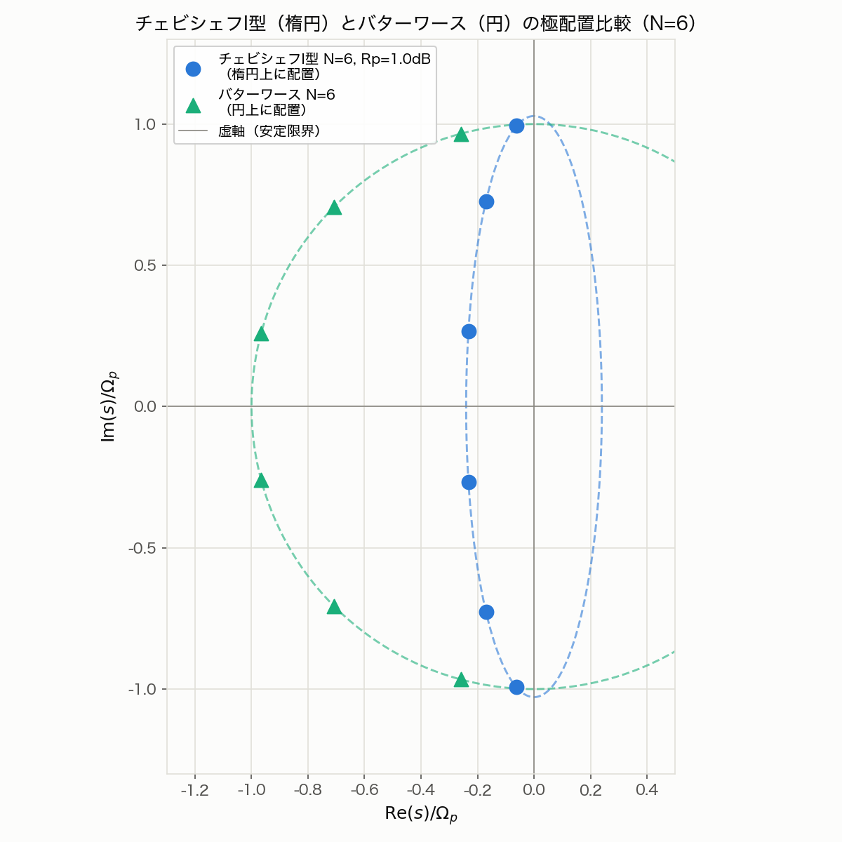
Edge case: poles approach the imaginary axis at high order / low ripple: the ellipse’s semi-minor axis is set by \(\sinh(v)=\sinh(\operatorname{arcsinh}(1/\varepsilon)/N)\) . As \(N\) grows or \(R_p\) (hence \(\varepsilon\) ) shrinks, \(v\to 0\) and \(\sinh(v)\approx v\) , so the pole’s real part (damping) shrinks as \(O(1/N)\) . In other words, high-order, low-ripple designs push the poles closer to the imaginary axis, raising the Q factor (resonance sharpness). In practice this makes direct-form transfer function coefficients more prone to catastrophic cancellation; as with the elliptic filter , second-order-sections (SOS) implementation is recommended for large \(N\) .
Chebyshev Type II Filter
The Chebyshev Type II (inverse Chebyshev) filter places equiripple in the stopband while maintaining a monotonic passband. Its magnitude squared function is:
\[|H(j\Omega)|^2 = \frac{1}{1 + \left[\varepsilon^2 T_N^2\!\left(\dfrac{\Omega_s}{\Omega}\right)\right]^{-1}} \tag{6}\]where \(\Omega_s\) is the stopband edge angular frequency. With a monotonic passband, the phase response is smoother than Type I.
Edge Case: cheby2’s Wn Parameter Marks the Stopband Edge
scipy.signal.cheby1 and scipy.signal.cheby2 both take a single “cutoff frequency” argument Wn, but it means something different for each type:
cheby1(N, rp, Wn, ...):Wnis \(\Omega_p\) from equation (2) — the passband edge, where gain reaches \(-R_p\) dBcheby2(N, rs, Wn, ...):Wnis \(\Omega_s\) from equation (6) — the stopband edge, where gain reaches \(-R_s\) dB
Because the argument shares the name Wn in both calls, it’s easy to assume “Wn = passband edge” out of habit from cheby1 and misuse it in cheby2. Let’s design a 6th-order Type II filter with stopband edge 150 Hz and stopband attenuation 40 dB, and check the gain at several frequencies.
import numpy as np
from scipy import signal

fs = 1000
N = 6
rs = 40.0
fs_stop = 150  # Wn passed to cheby2 is the "stopband edge" -- the point where gain reaches -rs

sos = signal.cheby2(N, rs, fs_stop, btype='low', fs=fs, output='sos')
freqs = np.array([50, 100, 130, 140, 149, 150, 160, 200])
_, h = signal.sosfreqz(sos, worN=freqs, fs=fs)
gdb = 20 * np.log10(np.abs(h))

for f, g in zip(freqs, gdb):
    print(f"f={f:4d} Hz  gain={g:8.3f} dB")
Output:
f=  50 Hz  gain=  -0.000 dB
f= 100 Hz  gain=  -0.759 dB
f= 130 Hz  gain= -15.531 dB
f= 140 Hz  gain= -24.903 dB
f= 149 Hz  gain= -37.759 dB
f= 150 Hz  gain= -40.000 dB
f= 160 Hz  gain= -43.434 dB
f= 200 Hz  gain= -66.189 dB
At the specified fs_stop=150 Hz the gain is exactly -rs=-40.0 dB, confirming that Wn marks the stopband edge. Equally notable: the passband already degrades well before Wn. At 100 Hz (two-thirds of the way to the stopband edge) the gain has already dropped by \(-0.759\)
dB — so assuming “flat up to Wn” is also a mistake. Chebyshev Type II has no passband-ripple parameter of its own and no explicit passband-edge argument, so “how far the passband stays effectively flat” depends on the transition-band shape set by the combination of \(N\)
, \(R_s\)
, and Wn. When the passband edge must be specified precisely, it’s safer to pass both edges to scipy.signal.cheb2ord and let it compute the order and Wn automatically.
Type I vs Type II Comparison
| Property | Chebyshev Type I | Chebyshev Type II |
|---|---|---|
| Passband | Equiripple | Monotone (flat) |
| Stopband | Monotone | Equiripple |
| Transition | Sharper than Butterworth | Sharper than Butterworth |
| Phase | Nonlinear | Relatively smooth |
| Use case | Sharp cutoff, ripple allowed | Flat passband, sharp cutoff |
Filter Order Determination
Given specifications (passband ripple \(R_p\) , stopband attenuation \(R_s\) , passband edge \(\Omega_p\) , stopband edge \(\Omega_s\) ), the minimum required order is:
\[N \geq \frac{\operatorname{arccosh}\!\left(\sqrt{\dfrac{10^{R_s/10}-1}{10^{R_p/10}-1}}\right)}{\operatorname{arccosh}(\Omega_s/\Omega_p)} \tag{7}\]For the same specification, a Chebyshev filter requires a lower order than a Butterworth filter.
Deriving equation (7)
At the stopband edge \(\Omega_s\) , meeting the required attenuation \(R_s\) [dB] means, in addition to the passband-based \(\varepsilon\) (equation 3), introducing a stopband analog
\[ \varepsilon_s = \sqrt{10^{R_s/10}-1} \]which lets us write the requirement as
\[ |H(j\Omega_s)|^2 = \frac{1}{1+\varepsilon^2 T_N^2(\Omega_s/\Omega_p)} \leq \frac{1}{1+\varepsilon_s^2} \]Comparing denominators,
\[ \varepsilon^2 T_N^2(\Omega_s/\Omega_p) \geq \varepsilon_s^2 \]Since the stopband edge lies above the passband edge (their ratio exceeds 1), \(T_N(x) = \cosh(N\operatorname{arccosh} x)\) is positive and strictly increasing there, so taking the square root directly gives
\[ T_N(\Omega_s/\Omega_p) \geq \frac{\varepsilon_s}{\varepsilon} \quad\Longleftrightarrow\quad \cosh\!\big(N\operatorname{arccosh}(\Omega_s/\Omega_p)\big) \geq \frac{\varepsilon_s}{\varepsilon} \]Applying \(\operatorname{arccosh}\) (monotone increasing) to both sides,
\[ N\operatorname{arccosh}(\Omega_s/\Omega_p) \geq \operatorname{arccosh}\!\left(\frac{\varepsilon_s}{\varepsilon}\right) \]hence
\[ N \geq \frac{\operatorname{arccosh}(\varepsilon_s/\varepsilon)}{\operatorname{arccosh}(\Omega_s/\Omega_p)} \]Substituting
\[ \frac{\varepsilon_s}{\varepsilon} = \sqrt{\frac{\varepsilon_s^2}{\varepsilon^2}} = \sqrt{\frac{10^{R_s/10}-1}{10^{R_p/10}-1}} \]recovers equation (7) exactly. Equality gives the exact real-valued order that just meets the specification, so the order actually used is the smallest integer at or above it (rounded up).
Python Implementation
Chebyshev Type I Filter with SciPy
import numpy as np
import matplotlib.pyplot as plt
from scipy import signal

# --- Filter specification ---
fs = 1000         # Sampling frequency [Hz]
fp = 100          # Passband edge [Hz]
rp = 1.0          # Passband ripple [dB]
orders = [2, 4, 6]

fig, axes = plt.subplots(2, 1, figsize=(10, 8))

for N in orders:
    sos = signal.cheby1(N, rp, fp, btype='low', fs=fs, output='sos')
    w, h = signal.sosfreqz(sos, worN=4096, fs=fs)

    axes[0].plot(w, 20 * np.log10(np.abs(h) + 1e-12), label=f'N={N}')
    axes[1].plot(w, np.degrees(np.unwrap(np.angle(h))), label=f'N={N}')

axes[0].set_xlabel('Frequency [Hz]')
axes[0].set_ylabel('Magnitude [dB]')
axes[0].set_title('Chebyshev Type I - Magnitude Response (rp=1dB)')
axes[0].set_xlim(0, 500)
axes[0].set_ylim(-80, 5)
axes[0].axvline(fp, color='gray', linestyle='--', alpha=0.5, label=f'fp={fp}Hz')
axes[0].axhline(-rp, color='r', linestyle=':', alpha=0.5, label=f'-{rp}dB ripple')
axes[0].legend()
axes[0].grid(True, alpha=0.3)

axes[1].set_xlabel('Frequency [Hz]')
axes[1].set_ylabel('Phase [degrees]')
axes[1].set_title('Chebyshev Type I - Phase Response')
axes[1].set_xlim(0, 500)
axes[1].legend()
axes[1].grid(True, alpha=0.3)

plt.tight_layout()
plt.show()
Chebyshev Type II Filter
import numpy as np
import matplotlib.pyplot as plt
from scipy import signal

fs = 1000
fs_stop = 150     # Stopband edge [Hz]
rs = 40.0         # Stopband attenuation [dB]
orders = [2, 4, 6]

fig, axes = plt.subplots(2, 1, figsize=(10, 8))

for N in orders:
    sos = signal.cheby2(N, rs, fs_stop, btype='low', fs=fs, output='sos')
    w, h = signal.sosfreqz(sos, worN=4096, fs=fs)

    axes[0].plot(w, 20 * np.log10(np.abs(h) + 1e-12), label=f'N={N}')
    axes[1].plot(w, np.degrees(np.unwrap(np.angle(h))), label=f'N={N}')

axes[0].set_xlabel('Frequency [Hz]')
axes[0].set_ylabel('Magnitude [dB]')
axes[0].set_title('Chebyshev Type II - Magnitude Response (rs=40dB)')
axes[0].set_xlim(0, 500)
axes[0].set_ylim(-80, 5)
axes[0].axvline(fs_stop, color='gray', linestyle='--', alpha=0.5, label=f'fs={fs_stop}Hz')
axes[0].axhline(-rs, color='r', linestyle=':', alpha=0.5, label=f'-{rs}dB')
axes[0].legend()
axes[0].grid(True, alpha=0.3)

axes[1].set_xlabel('Frequency [Hz]')
axes[1].set_ylabel('Phase [degrees]')
axes[1].set_title('Chebyshev Type II - Phase Response')
axes[1].set_xlim(0, 500)
axes[1].legend()
axes[1].grid(True, alpha=0.3)

plt.tight_layout()
plt.show()
Order Comparison with Butterworth
from scipy.signal import buttord, cheb1ord, cheb2ord

fp = 100       # Passband edge [Hz]
fs_stop = 150  # Stopband edge [Hz]
rp = 1.0       # Passband ripple [dB]
rs = 40.0      # Stopband attenuation [dB]
fs = 1000      # Sampling frequency

N_butter, Wn_butter = buttord(fp, fs_stop, rp, rs, fs=fs)
N_cheby1, Wn_cheby1 = cheb1ord(fp, fs_stop, rp, rs, fs=fs)
N_cheby2, Wn_cheby2 = cheb2ord(fp, fs_stop, rp, rs, fs=fs)

print(f"Butterworth    : order {N_butter}")
print(f"Chebyshev I    : order {N_cheby1}")
print(f"Chebyshev II   : order {N_cheby2}")
Output:
Butterworth    : order 12
Chebyshev I    : order 6
Chebyshev II   : order 6
For the same specification (passband edge 100 Hz, stopband edge 150 Hz, passband ripple 1 dB, stopband attenuation 40 dB), Butterworth needs order 12 while both Chebyshev types need only order 6. Since order directly sets the number of transfer-function state variables (i.e. implementation cost), Chebyshev achieves the same spec here at half the computation/memory of Butterworth.
Let’s verify this order-6 Chebyshev Type I filter actually meets the specification.
from scipy import signal
import numpy as np

sos1 = signal.cheby1(N_cheby1, rp, Wn_cheby1, btype='low', fs=fs, output='sos')
_, h = signal.sosfreqz(sos1, worN=[fp, fs_stop], fs=fs)
gdb = 20 * np.log10(np.abs(h))
print(f"cheby1 N={N_cheby1}: gain@fp={gdb[0]:.3f}dB (require -{rp}dB), gain@fs_stop={gdb[1]:.3f}dB (require <=-{rs}dB)")
Output:
cheby1 N=6: gain@fp=-1.000dB (require -1.0dB), gain@fs_stop=-41.324dB (require <=-40.0dB)
At the passband edge the gain is exactly \(-1.000\) dB as required, and at the stopband edge it reaches \(-41.324\) dB against a \(-40.0\) dB requirement — over 1.3 dB of margin. See the elliptic filter article for a side-by-side order comparison across Butterworth, Chebyshev I, Chebyshev II, and elliptic (which achieves an even lower order under the same specification).
Noise Reduction Application
import numpy as np
import matplotlib.pyplot as plt
from scipy import signal

fs = 1000
t = np.arange(0, 1, 1/fs)
clean = np.sin(2 * np.pi * 10 * t) + 0.5 * np.sin(2 * np.pi * 30 * t)
noisy = clean + 0.8 * np.random.randn(len(t))

# Butterworth (order 4)
sos_butter = signal.butter(4, 100, fs=fs, output='sos')
y_butter = signal.sosfiltfilt(sos_butter, noisy)

# Chebyshev Type I (order 4, 1 dB ripple)
sos_cheby1 = signal.cheby1(4, 1, 100, fs=fs, output='sos')
y_cheby1 = signal.sosfiltfilt(sos_cheby1, noisy)

# Chebyshev Type II (order 4, 40 dB attenuation)
sos_cheby2 = signal.cheby2(4, 40, 150, fs=fs, output='sos')
y_cheby2 = signal.sosfiltfilt(sos_cheby2, noisy)

fig, axes = plt.subplots(4, 1, figsize=(10, 12), sharex=True)
axes[0].plot(t, noisy, alpha=0.5, label='Noisy'); axes[0].plot(t, clean, 'k', label='Original')
axes[0].set_title('Input Signal'); axes[0].legend(); axes[0].grid(True, alpha=0.3)

axes[1].plot(t, y_butter, label='Butterworth N=4'); axes[1].plot(t, clean, 'k', lw=1.5)
axes[1].set_title('Butterworth (N=4)'); axes[1].legend(); axes[1].grid(True, alpha=0.3)

axes[2].plot(t, y_cheby1, label='Chebyshev I N=4, rp=1dB'); axes[2].plot(t, clean, 'k', lw=1.5)
axes[2].set_title('Chebyshev Type I (N=4, rp=1dB)'); axes[2].legend(); axes[2].grid(True, alpha=0.3)

axes[3].plot(t, y_cheby2, label='Chebyshev II N=4, rs=40dB'); axes[3].plot(t, clean, 'k', lw=1.5)
axes[3].set_title('Chebyshev Type II (N=4, rs=40dB)')
axes[3].set_xlabel('Time [s]'); axes[3].legend(); axes[3].grid(True, alpha=0.3)

plt.tight_layout()
plt.show()
Comparison with Other IIR Filters
| Filter | Passband | Stopband | Transition | Phase |
|---|---|---|---|---|
| Butterworth | Maximally flat | Monotone | Wide | Relatively smooth |
| Chebyshev Type I | Equiripple | Monotone | Narrower | Nonlinear |
| Chebyshev Type II | Monotone | Equiripple | Narrower | Relatively smooth |
| Elliptic (Cauer) | Equiripple | Equiripple | Narrowest | Most nonlinear |
Use Type I when a sharp cutoff is needed and passband ripple is acceptable. Use Type II when passband flatness is required but improved stopband attenuation is desired.
Recent Research
The classical integer-order Chebyshev filter, established since the 1930s, meets its three specifications — passband ripple, stopband attenuation, and transition width — via the closed forms in equations (2), (6), and (7). But the order \(N\) can only be an integer, so a requirement that falls between “order \(N\) is barely insufficient” and “order \(N+1\) is overkill” forces you to spend an entire extra order. In 2024, Daryani and Aggarwal addressed this by treating the order as a continuous real number \(1+\alpha\) (\(0<\alpha<1\) ) in a fractional-order Chebyshev lowpass filter, applying nature-inspired metaheuristic optimization — particle swarm optimization (PSO), the firefly algorithm (FA), and grey wolf optimization (GWO) — to find coefficients that closely track the ideal fractional-order Chebyshev response. They further realized these coefficients in analog circuit topologies based on OTAs (operational transconductance amplifiers) and CCIIs (second-generation current conveyors), and SPICE simulation confirmed mean-square errors against the ideal response of \(-48.67\) dB (CCII) and \(-62.8\) dB (OTA) (Daryani & Aggarwal, 2024, Integration, the VLSI Journal).
This work does not replace the integer-order Type I design covered in this article — it’s an extension that continuizes the discrete order parameter to reach “in-between” transition sharpness that integer orders cannot express. For embedded applications tightly constrained to a fixed integer order, the classical design in this article remains the mainstream choice; but for analog circuit design, or research contexts that want to treat order itself as a continuous optimization parameter, the fractional-order approach may become an increasingly available option.
Summary
- Chebyshev filters exploit the equal-amplitude oscillation property of Chebyshev polynomials to produce equiripple IIR filters
- Type I has equiripple in the passband; Type II has equiripple in the stopband
- The Chebyshev polynomial is chosen as the equiripple building block because it uniquely minimizes the sup norm among monic polynomials on \([-1,1]\) (the minimax / equioscillation theorem)
- Type I’s DC gain depends on order parity: exactly 0 dB for odd orders, exactly \(-R_p\) dB for even orders
- Both types achieve sharper transition bands than Butterworth at the same order (in this article’s worked example: order 12 for Butterworth vs. order 6 for both Chebyshev types)
- In SciPy, use
signal.cheby1()/signal.cheby2()for design, andsignal.cheb1ord()/signal.cheb2ord()to compute the required order automatically
Related Articles
- Lowpass Filter Design: Moving Average, Butterworth, and Chebyshev - Compares all three filter types by frequency response, group delay, and step response.
- Butterworth Filter Design: Theory and Python Implementation - The maximally flat IIR filter, a close relative of the Chebyshev.
- FIR vs IIR Filters - Design philosophy differences between Chebyshev (IIR) and FIR filters.
- Notch Filter Design and Python Implementation - Applying IIR filter design to remove a specific frequency.
- Exponential Moving Average (EMA) Filter: Frequency Characteristics - The simplest 1st-order IIR filter as a stepping stone to Chebyshev.
- Fast Fourier Transform (FFT): Theory and Python Implementation - Analyzing filter frequency responses with FFT.
- Bessel Filter: Theory and Python Implementation - Sister IIR with a much gentler roll-off but nearly flat group delay — chosen when minimizing phase distortion matters more than transition steepness.
- Elliptic (Cauer) Filter: Theory and Python Implementation - Allows ripple in both pass and stop bands and achieves the steepest transition for a given order — Chebyshev taken to its logical extreme.
- Bandpass Filter Design: Theory and Python Implementation — Apply the Chebyshev prototype to bandpass design when in-band ripple is acceptable in exchange for sharper transition.
- Filter Design Selection Guide: 3 axes and characteristic comparison — Use this hub to position the Chebyshev filter against alternatives during selection.
References
- Chebyshev, P. L. (1854). Théorie des mécanismes connus sous le nom de parallélogrammes. Mémoires des Savants Étrangers présentés à l’Académie de Saint-Pétersbourg, 7, 539-586.
- Proakis, J. G., & Manolakis, D. G. (2007). Digital Signal Processing (4th ed.). Pearson.
- Oppenheim, A. V., & Schafer, R. W. (2009). Discrete-Time Signal Processing (3rd ed.). Prentice Hall.
- Daryani, R., & Aggarwal, B. (2024). Nature inspired algorithm based design of near ideal fractional order low pass Chebyshev filters and their realization using OTAs and CCII. Integration, the VLSI Journal, 97, 102185. https://doi.org/10.1016/j.vlsi.2024.102185
- SciPy scipy.signal.cheby1 documentation
- SciPy scipy.signal.cheby2 documentation
- SciPy scipy.signal.cheb1ap documentation