Introduction
The elliptic filter (also known as the Cauer filter) is an IIR filter that exhibits equiripple behavior in both the passband and the stopband. Among all IIR filters of the same order, it achieves the steepest transition band:
\[\text{Elliptic} > \text{Chebyshev (Type I \& II)} > \text{Butterworth}\]The trade-off is that both the passband and stopband contain ripples. This article covers the mathematical background and practical design using SciPy.
This dual-band equiripple property traces back to a problem solved in 1877 by the Russian mathematician Yegor Zolotarev (1847–1878), a student of Chebyshev: the best uniform rational approximation on two separated intervals of the real line, now known as the Zolotarev problem. Zolotarev learned elliptic function theory from Weierstrass during a visit to Berlin and applied it to solve this problem. The first application of this solution to electrical filter design was by Wilhelm Cauer in 1933 — hence the alternative name “Cauer filter.”
Frequency Response
The squared magnitude response of an elliptic filter is:
\[|H(j\Omega)|^2 = \frac{1}{1 + \varepsilon^2 R_n^2(\xi, \Omega/\Omega_p)} \tag{1}\]where:
- \(\varepsilon\) : passband ripple parameter (\(\varepsilon^2 = 10^{R_p/10} - 1\) )
- \(R_n(\xi, x)\) : Jacobi elliptic rational function of order \(n\)
- \(\xi\) : selectivity parameter (\(\xi = \Omega_p / \Omega_s > 1\) )
- \(n\) : filter order
Jacobi Elliptic Rational Function: Why Both Bands Become Equiripple
Type I Chebyshev filters achieve passband equiripple using the Chebyshev polynomial \(T_n(x) = \cos(n \arccos x)\) . The crux of this construction is the substitution \(x = \cos\theta\) . As long as \(\theta\) is real, \(\cos\) has only a single real period (\(2\pi\) ), so for \(|x| \le 1\) (real \(\theta\) ) it oscillates with equal amplitude, but for \(|x| > 1\) , \(\theta\) becomes purely imaginary and \(\cos\theta \to \cosh u\) , which grows monotonically. This is exactly why Chebyshev Type I’s stopband can only be monotonically decreasing. Type II applies the same construction to the reciprocal variable \(\Omega_s/\Omega\) , moving the equiripple region to the stopband — but the passband then becomes monotonic. Either way, the same trigonometric substitution can only deliver equiripple behavior on one side, never both.
The elliptic filter breaks this constraint simultaneously. Achieving equiripple on both \(|x|\le 1\) and \(|x|\ge \xi\) requires replacing \(\cos\theta\) (a function with only a single real period) with a substitution based on a doubly-periodic (elliptic) function, which has both a real and an imaginary period. The Jacobi elliptic function \(\text{sn}(u,k)\) has a real period \(4K(k)\) and an imaginary period \(2iK'(k)\) (where \(K'(k)=K(\sqrt{1-k^2})\) is the complementary complete elliptic integral); the periodicity along the real axis produces the passband ripple, while the periodicity along the imaginary axis produces the stopband ripple. Using this double periodicity, one constructs the degree-\(n\) rational function
\[ R_n(\xi, x) = \text{cd}\!\left(n\, \frac{K(1/\xi)}{K(k)}\, \text{cd}^{-1}(x, k),\ k\right) \](where \(\text{cd} = \text{cn}/\text{dn}\) is a Jacobi elliptic function, and \(k\) is a modulus determined by \(\xi\) ), which satisfies:
- \(|x| \le 1 \Rightarrow |R_n(\xi, x)| \le 1\) , oscillating with equal amplitude \(n\) times inside the interval (passband equiripple)
- \(|x| \ge \xi \Rightarrow |R_n(\xi, x)| \ge \xi\) , oscillating with equal amplitude inside the interval (stopband equiripple)
This \(R_n(\xi,x)\) is the Zolotarev rational function — a generalization of Chebyshev’s “single-period, polynomial” equiripple theory to a “doubly-periodic, rational-function” setting (Orfanidis, 2006). Substituting this \(R_n\) into eq. (1) yields an elliptic filter’s amplitude response with equiripple behavior in both bands.
Order Determination
The minimum order required to meet specifications (\(\Omega_p\) , \(\Omega_s\) , \(R_p\) , \(R_s\) ) is:
\[n \ge \frac{K(1/\xi) \cdot K(\sqrt{1-1/\xi_s^2})}{K(\xi_s) \cdot K(\sqrt{1-1/\xi^2})} \tag{2}\]where \(K(\cdot)\)
is the complete elliptic integral of the first kind. In practice, scipy.signal.ellipord computes this automatically.
Deriving Eq. (2): The Order Formula via the Elliptic Nome
We can derive why eq. (2) holds using a quantity called the nome of an elliptic function. Define:
- Selectivity factor: \(k = \Omega_p / \Omega_s\) (\(0 < k < 1\) ; corresponds to \(1/\xi\) in eq. (2))
- Discrimination factor:
- Complementary modulus \(k' = \sqrt{1-k^2}\) , \(K'(k) = K(k')\)
- Elliptic nome: \(q(k) = \exp(-\pi K'(k)/K(k))\)
The Zolotarev rational function \(R_n(\xi,x)\) from the previous section maps an “input” configuration with modulus \(k\) to an “output” configuration with modulus \(k_1\) through an \(n\) -fold composition. This \(n\) -fold composition is the elliptic-function analogue of the repeated double-angle identity \(\cos(n\theta) = T_n(\cos\theta)\) (equivalent to \(n\) applications of the Landen transformation), and acting on the nome it takes the simple form of a power law:
\[q(k_1) = \big[q(k)\big]^{\,n}\](Orfanidis, 2006). Solving this for \(n\) gives:
\[ n = \frac{\ln q(k_1)}{\ln q(k)} = \frac{K(k)\, K'(k_1)}{K'(k)\, K(k_1)} \]which matches eq. (2) once we substitute \(\xi = 1/k\) and \(\xi_s = 1/k_1\) . Since equality gives the (real-valued) order that exactly meets specifications, the order actually used is the smallest integer \(\ge n\) (i.e., \(\lceil n \rceil\) ).
Numerical verification: for \(f_p=100\)
Hz, \(f_s=150\)
Hz, \(R_p=1\)
dB, \(R_s=60\)
dB, we have \(k = 100/150 = 0.6667\)
, \(\varepsilon = 0.5088\)
, \(\varepsilon_1 = 999.9995\)
, giving \(k_1 = \varepsilon/\varepsilon_1 = 5.088 \times 10^{-4}\)
. Computing \(K, K'\)
with scipy.special.ellipk:
import numpy as np
from scipy.special import ellipk
from scipy import signal

rp, rs = 1.0, 60.0
fp, fs_stop = 100, 150

eps  = np.sqrt(10**(rp/10) - 1)
eps1 = np.sqrt(10**(rs/10) - 1)
k  = fp / fs_stop
k1 = eps / eps1

def K(m):
    return ellipk(m**2)  # scipy.special.ellipk takes m = k^2

Kk, Kpk   = K(k),  K(np.sqrt(1 - k**2))
Kk1, Kpk1 = K(k1), K(np.sqrt(1 - k1**2))

n_formula = (Kk * Kpk1) / (Kpk * Kk1)
print(f"k={k:.4f}  k1={k1:.6e}")
print(f"n (real-valued) = {n_formula:.4f}  -> order used = {int(np.ceil(n_formula))}")

n_ellipord, _ = signal.ellipord(fp/500, fs_stop/500, rp, rs)
print(f"order from scipy.signal.ellipord = {n_ellipord}")
Output:
k=0.6667  k1=5.088473e-04
n (real-valued) = 5.4267  -> order used = 6
order from scipy.signal.ellipord = 6
The theoretical value \(n=5.4267\)
from eq. (2) (derived from the nome power law), rounded up to order 6, matches exactly the order 6 actually returned by scipy.signal.ellipord.
Pole/Zero Placement: Finite Transmission Zeros
The steep transition band is achieved through the zero placement of the transfer function \(H(s)\) . Because the Zolotarev rational function \(R_n(\xi,x)\) vanishes at finite points \(x=\xi_1, \xi_2,\dots\) (points at or beyond \(\xi\) ), the corresponding \(H(s)\) has zeros at finite points \(s=j\Omega_1, j\Omega_2,\dots\) on the imaginary axis. These are called finite transmission zeros. At each such frequency the gain is theoretically \(-\infty\) dB, and these deep notches are precisely what create the stopband equiripple valleys.
It’s worth noting that Butterworth, Chebyshev Type I, Chebyshev Type II, and elliptic filters do not all share the same zero structure. Let’s check with SciPy’s analog-prototype functions.
from scipy import signal

N = 6
z_butter, _, _ = signal.buttap(N)
z_cheby1, _, _ = signal.cheb1ap(N, 1.0)
z_cheby2, _, _ = signal.cheb2ap(N, 60.0)
z_ellip,  _, _ = signal.ellipap(N, 1.0, 60.0)

print("Butterworth  finite zero count:", len(z_butter))
print("Chebyshev I  finite zero count:", len(z_cheby1))
print("Chebyshev II finite zero count:", len(z_cheby2))
print("Elliptic     finite zero count:", len(z_ellip))
Output:
Butterworth  finite zero count: 0
Chebyshev I  finite zero count: 0
Chebyshev II finite zero count: 6
Elliptic     finite zero count: 6
Butterworth and Chebyshev Type I build their amplitude response from a polynomial (\(T_n\) itself), so they have no finite zeros — all zeros sit at \(s=\infty\) (one reason their stopbands can only decay monotonically). Chebyshev Type II, on the other hand, applies the Type I construction to a reciprocal variable, making it a rational function — and it therefore has finite zeros in its stopband, just like the elliptic filter. In other words, the real dividing line for “does it have finite transmission zeros” is not “Butterworth/Chebyshev vs. elliptic” but “polynomial approximation (Butterworth, Chebyshev I) vs. rational-function approximation (Chebyshev II, elliptic).” What makes the elliptic filter special is that it applies this rational-function approximation to both bands simultaneously, making both sides equiripple.
The count of finite transmission zeros also has an even/odd-order edge case. For an \(n\) -th order elliptic filter, the number of finite zero pairs is \(n/2\) when \(n\) is even (every pole pair has a matching finite zero), and \((n-1)/2\) when \(n\) is odd (one pole has no matching finite zero and effectively sits at \(s=\infty\) ).
from scipy import signal
for N in [5, 6, 7]:
    z, p, k = signal.ellipap(N, 1.0, 60.0)
    print(f"n={N}: poles={len(p)}  finite zeros={len(z)}")
n=5: poles=5  finite zeros=4
n=6: poles=6  finite zeros=6
n=7: poles=7  finite zeros=6
This asymmetry has an important practical consequence. For even orders, the number of zero pairs equals the number of pole pairs, so as \(\Omega\to\infty\) the gain asymptotes to the stopband ripple floor (\(-R_s\) dB) and goes no lower. For odd orders, one extra pole means the gain keeps decaying monotonically beyond the last finite zero.
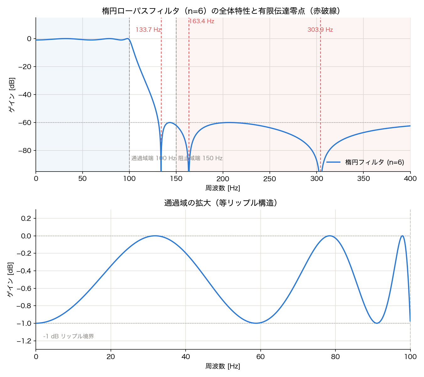
Let’s compute and visualize the finite transmission-zero frequencies for \(n=6\)
(the order returned by scipy.signal.ellipord(100, 150, 1, 60, fs=1000)).
import numpy as np
from scipy import signal

fs = 1000
rp, rs = 1.0, 60.0
n, wn = signal.ellipord(100, 150, rp, rs, fs=fs)  # keep everything in Hz (wn is also in Hz when fs= is passed)

z, p, k = signal.ellip(n, rp, rs, wn, btype='low', fs=fs, output='zpk')
b, a = signal.zpk2tf(z, p, k)

print("Zero magnitudes (checking unit circle):", np.round(np.abs(z), 6))

# Evaluate H(z) exactly at each zero's own angular frequency to confirm the depth
uniq_ang = sorted(set(round(abs(np.angle(zz)), 10) for zz in z))
_, h_exact = signal.freqz(b, a, worN=np.array(uniq_ang))
for wa, hh in zip(uniq_ang, h_exact):
    f_hz = wa * fs / (2 * np.pi)
    print(f"f={f_hz:6.2f} Hz   |H|={abs(hh):.2e}   ({20*np.log10(abs(hh)+1e-300):.1f} dB)")
Output:
Zero magnitudes (checking unit circle): [1. 1. 1. 1. 1. 1.]
f=133.73 Hz   |H|=1.31e-12   (-237.6 dB)
f=163.41 Hz   |H|=3.02e-13   (-250.4 dB)
f=303.88 Hz   |H|=1.85e-14   (-274.6 dB)
Every zero lies on the unit circle (\(|z|=1\)
, i.e., on the imaginary axis analytically), and the 3 finite zero pairs are distributed from just past the passband/stopband edges (100 Hz / 150 Hz) across the stopband. The theoretical gain there is \(-\infty\)
dB, but due to floating-point rounding the measured depth is around \(-238\)
to \(-275\)
dB — effectively infinite for any practical purpose. Interestingly, the first zero (133.73 Hz) falls inside the nominal transition band, before the specified stopband edge of 150 Hz. This is because ellipord only guarantees “at least \(R_s\)
dB of attenuation from 150 Hz onward” — it does not forbid the attenuation from momentarily dipping even deeper before that point.
The figure below shows the overall response of this elliptic filter (\(n=6\) ) (top) alongside a zoomed view of the passband’s equiripple structure (bottom). The red dashed lines in the top panel mark the finite transmission zeros, each coinciding with the bottom of a stopband ripple valley.
Comparison with Butterworth and Chebyshev
| Filter | Passband | Stopband | Transition Band (same order) | Phase Response |
|---|---|---|---|---|
| Butterworth | Maximally flat | Monotone | Widest | Best |
| Chebyshev Type I | Equiripple | Monotone | Moderate | Moderate |
| Chebyshev Type II | Maximally flat | Equiripple | Moderate | Moderate |
| Elliptic | Equiripple | Equiripple | Narrowest | Worst |
The elliptic filter maximizes transition band steepness at the cost of nonlinear phase response (poor group delay flatness).
Group Delay and the Pulse-Response Trade-off
Let’s quantify the cost of the steep amplitude response. Group delay is the negative derivative of the phase response with respect to frequency:
\[\tau(\omega) = -\frac{d\phi(\omega)}{d\omega}\]If group delay is constant across frequency, the filter has linear phase and preserves pulse waveform shape. The Bessel filter is designed to make this group delay as flat as possible in the passband — the exact opposite design philosophy from the elliptic filter. The elliptic filter introduces rapid phase rotation near the passband edge (a consequence of its rational-function construction), causing large group-delay variation there.
Let’s measure the passband (1–90 Hz) group-delay variation and the unit-step-response overshoot for Butterworth, Chebyshev I, Elliptic, and Bessel filters, all at the same order (\(n=4\) ).
import numpy as np
from scipy import signal

fs = 1000
fc = 100
N = 4
rp, rs = 1.0, 60.0

filters = {
    'Butterworth': signal.butter(N, fc, btype='low', fs=fs),
    'Chebyshev I': signal.cheby1(N, rp, fc, btype='low', fs=fs),
    'Elliptic':    signal.ellip(N, rp, rs, fc, btype='low', fs=fs),
    'Bessel':      signal.bessel(N, fc, btype='low', fs=fs, norm='delay'),
}

print("=== Passband (1-90Hz) group delay variation ===")
for name, ba in filters.items():
    w, gd_samples = signal.group_delay(ba, w=4096, fs=fs)
    gd_ms = gd_samples / fs * 1000.0          # samples -> milliseconds
    mask = (w >= 1) & (w <= 90)
    gd = gd_ms[mask]
    print(f"{name:12s}: mean={gd.mean():.3f}ms  "
          f"min={gd.min():.3f}ms  max={gd.max():.3f}ms  "
          f"variation={(gd.max()-gd.min()):.3f}ms")

print()
print("=== Unit step response overshoot ===")
for name, ba in filters.items():
    b, a = ba
    t = np.arange(0, 0.3, 1/fs)
    y = signal.lfilter(b, a, np.ones(len(t)))
    steady = y[-50:].mean()
    overshoot = (y.max() - steady) / steady * 100
    print(f"{name:12s}: steady={steady:.4f}  peak={y.max():.4f}  overshoot={overshoot:.2f}%")
Output:
=== Passband (1-90Hz) group delay variation ===
Butterworth : mean=4.848ms  min=4.021ms  max=6.522ms  variation=2.501ms
Chebyshev I : mean=5.697ms  min=4.148ms  max=10.450ms  variation=6.302ms
Elliptic    : mean=5.539ms  min=3.903ms  max=10.598ms  variation=6.694ms
Bessel      : mean=1.582ms  min=1.539ms  max=1.669ms  variation=0.130ms

=== Unit step response overshoot ===
Butterworth : steady=1.0000  peak=1.1191  overshoot=11.91%
Chebyshev I : steady=0.8913  peak=1.0923  overshoot=22.56%
Elliptic    : steady=0.8913  peak=1.1017  overshoot=23.61%
Bessel      : steady=1.0000  peak=1.0807  overshoot=8.07%
Even at the same 4th order, the passband group-delay variation is 0.130 ms for Bessel versus 6.694 ms for elliptic — more than 50x larger. This confirms with actual numbers the qualitative “phase response: worst” entry in the table above. Step-response overshoot is likewise largest for elliptic (23.61%) versus Bessel’s 8.07%, showing that the steep amplitude response comes at the cost of strong ringing (oscillatory overshoot) on rectangular-type inputs. Note that Chebyshev I (equiripple passband only) and Elliptic (equiripple both bands) land close together here, suggesting that passband non-flatness itself is the dominant driver of the deviation from linear phase. For applications where waveform preservation is paramount (measurement instruments, pulse transmission), avoid the elliptic filter and choose Bessel instead.
SciPy Implementation
import numpy as np
import matplotlib.pyplot as plt
from scipy import signal

# ===== Design Parameters =====
fs = 1000          # Sampling frequency [Hz]
f_pass = 100       # Passband edge [Hz]
f_stop = 150       # Stopband edge [Hz]
rp = 1.0           # Passband ripple [dB]
rs = 60.0          # Stopband attenuation [dB]

# Normalize to Nyquist frequency
nyq = fs / 2
wp = f_pass / nyq
ws = f_stop / nyq

# ===== Compute Minimum Order =====
n, wn = signal.ellipord(wp, ws, rp, rs)
print(f"Minimum elliptic filter order: {n}")

# ===== Design Lowpass Elliptic Filter =====
b, a = signal.ellip(n, rp, rs, wn, btype='low')

# ===== Compute Frequency Response =====
w, h = signal.freqz(b, a, worN=2048, fs=fs)

# ===== Plot =====
fig, axes = plt.subplots(2, 1, figsize=(10, 8))

# Magnitude response
axes[0].plot(w, 20 * np.log10(np.abs(h)), label=f'Elliptic (n={n})', color='royalblue')
axes[0].axvline(f_pass, color='green', linestyle='--', alpha=0.7, label=f'Passband edge {f_pass}Hz')
axes[0].axvline(f_stop, color='red', linestyle='--', alpha=0.7, label=f'Stopband edge {f_stop}Hz')
axes[0].axhline(-rp, color='orange', linestyle=':', alpha=0.7, label=f'Ripple -{rp}dB')
axes[0].axhline(-rs, color='purple', linestyle=':', alpha=0.7, label=f'Attenuation -{rs}dB')
axes[0].set_ylim(-80, 5)
axes[0].set_xlabel('Frequency [Hz]')
axes[0].set_ylabel('Gain [dB]')
axes[0].set_title('Elliptic Filter: Magnitude Response')
axes[0].legend()
axes[0].grid(True)

# Phase response
angles = np.unwrap(np.angle(h))
axes[1].plot(w, np.degrees(angles), color='royalblue')
axes[1].set_xlabel('Frequency [Hz]')
axes[1].set_ylabel('Phase [degrees]')
axes[1].set_title('Elliptic Filter: Phase Response')
axes[1].grid(True)

plt.tight_layout()
plt.show()
Order Comparison Across Filter Types
Using the same specification (\(f_p=100\) Hz, \(f_s=150\) Hz, \(R_p=1\) dB, \(R_s=60\) dB):
from scipy import signal

fs = 1000
nyq = fs / 2
wp = 100 / nyq
ws = 150 / nyq
rp, rs = 1.0, 60.0

n_butter, _ = signal.buttord(wp, ws, rp, rs)
n_cheby1, _ = signal.cheb1ord(wp, ws, rp, rs)
n_cheby2, _ = signal.cheb2ord(wp, ws, rp, rs)
n_ellip, _ = signal.ellipord(wp, ws, rp, rs)

print(f"Butterworth  : order {n_butter}")
print(f"Chebyshev I  : order {n_cheby1}")
print(f"Chebyshev II : order {n_cheby2}")
print(f"Elliptic     : order {n_ellip}")
Actual output (SciPy 1.18.0):
Butterworth  : order 17
Chebyshev I  : order 9
Chebyshev II : order 9
Elliptic     : order 6
The elliptic filter achieves the same specification with less than 1/3 the order of a Butterworth filter. Order translates almost directly into the degree of the transfer function’s denominator polynomial — i.e., the required computation and number of state variables (memory) — so on resource-constrained embedded platforms this order gap is a direct implementation-cost gap. This order-6 result also matches exactly the ceiling of the theoretical value \(n=5.4267\) derived from the nome power law in eq. (2) above.
Highpass, Bandpass, and Bandstop Design
from scipy import signal

fs = 1000
nyq = fs / 2
rp, rs = 1.0, 60.0

# ===== Highpass Filter =====
n_hp, wn_hp = signal.ellipord(200/nyq, 100/nyq, rp, rs)
b_hp, a_hp = signal.ellip(n_hp, rp, rs, wn_hp, btype='high')

# ===== Bandpass Filter =====
n_bp, wn_bp = signal.ellipord(
    [100/nyq, 300/nyq], [50/nyq, 400/nyq], rp, rs
)
b_bp, a_bp = signal.ellip(n_bp, rp, rs, wn_bp, btype='bandpass')

# ===== Bandstop Filter =====
n_bs, wn_bs = signal.ellipord(
    [50/nyq, 400/nyq], [100/nyq, 300/nyq], rp, rs
)
b_bs, a_bs = signal.ellip(n_bs, rp, rs, wn_bs, btype='bandstop')
Numerical Stability: Use SOS Format
For higher-order filters (roughly n > 6), direct-form coefficients (b, a) can suffer from numerical precision issues. Use Second-Order Sections (SOS) format instead:
# SOS format: more numerically stable
sos = signal.ellip(n, rp, rs, wn, btype='low', output='sos')

# Zero-phase filtering (offline use)
y = signal.sosfiltfilt(sos, x)

# Causal filtering (real-time use)
y = signal.sosfilt(sos, x)
| Function | Phase delay | Real-time | Recommended when |
|---|---|---|---|
signal.lfilter | Yes | Yes | Real-time, low-order filters |
signal.filtfilt | None (zero-phase) | No | Offline analysis |
signal.sosfilt | Yes | Yes | Higher-order, real-time |
signal.sosfiltfilt | None | No | Higher-order, offline |
When to Choose Elliptic Filters
| Scenario | Recommended Filter |
|---|---|
| Steepest possible transition band | Elliptic |
| Minimize filter order (computation cost) | Elliptic |
| Passband ripple must be zero | Chebyshev Type II or Butterworth |
| Flat group delay (linear phase) | Butterworth or Bessel |
| Low latency real-time processing | Butterworth (low order) |
Recent Research Trends
Classical analog-prototype design (Butterworth, Chebyshev, elliptic, Bessel) remains the standard approach in signal processing, audio hardware, and communication systems for meeting a fixed set of specifications — passband ripple, stopband attenuation, and transition bandwidth — with a closed-form solution. This is exactly the design SciPy and MATLAB provide.
Since around 2023, however, research has increasingly explored embedding the basic IIR building block (especially the second-order section, or biquad) inside deep-learning pipelines. Lutati, Zimerman, and Wolf (EMNLP 2023), “Focus Your Attention (with Adaptive IIR Filters),” use input-dependent (adaptive) second-order IIR filters as a preprocessing layer ahead of attention, improving efficiency on long-sequence tasks. Separately, Malek, Schulz, and Wuebbelmann (DAFx25, 2025) report using Kolmogorov-Arnold Networks (KANs) to directly optimize biquad filter coefficients via learning.
It’s important not to read these as replacing the classical design covered in this article — deriving a minimum-order closed-form solution from given passband/stopband specifications. Rather, they represent a direction where the IIR filter structure itself becomes a learnable building block inside a neural network, freed from a fixed specification. At present, classical analog-prototype design and neural-network-based approaches seem less like competitors and more like complementary techniques suited to different settings — fixed frequency-domain specifications versus input-dependent, task-dependent adaptive behavior.
Related Articles
- Butterworth Filter Design and Python Implementation - Maximally flat IIR filter design
- Chebyshev Filter Design and Python Implementation - Equiripple IIR filter design
- FIR vs IIR Filter Comparison - Overview of IIR filter characteristics
- Lowpass Filter Design Comparison - Comparing various lowpass filter types
- Highpass Filter Design and Python Implementation - Highpass filter design
- Bandpass Filter Design and Python Implementation - Bandpass and bandstop filter design
- Notch Filter Design and Python Implementation - Narrow-band rejection filter design
- Exponential Moving Average (EMA) Filter Frequency Response - EMA as a first-order IIR filter
- Bessel Filter: Theory and Python Implementation - The opposite design philosophy from Elliptic — maximizes flat group delay rather than transition steepness.
- Filter Design Selection Guide: 3 axes and characteristic comparison — Use this hub to position the Elliptic filter against alternatives during selection.
References
- Zolotarev, E. I. (1877). Application of elliptic functions to questions of functions deviating least and most from zero. Zapiski Imperatorskoi Akademii Nauk, 30(5), 1-71.
- Cauer, W. (1933). Ein Interpolationsproblem mit Funktionen mit positivem Realteil. Mathematische Zeitschrift, 38, 1-44.
- Orfanidis, S. J. (2006). Lecture Notes on Elliptic Filter Design. Rutgers University, Department of Electrical & Computer Engineering.
- Proakis, J. G., & Manolakis, D. G. (2007). Digital Signal Processing (4th ed.). Pearson.
- Oppenheim, A. V., & Schafer, R. W. (2009). Discrete-Time Signal Processing (3rd ed.). Prentice Hall.
- Lutati, S., Zimerman, I., & Wolf, L. (2023). Focus Your Attention (with Adaptive IIR Filters). Proceedings of EMNLP 2023.
- Malek, A., Schulz, D., & Wuebbelmann, F. (2025). Biquad Coefficients Optimization via Kolmogorov-Arnold Networks. Proceedings of the 28th International Conference on Digital Audio Effects (DAFx25).
- SciPy scipy.signal.ellip documentation
- SciPy scipy.signal.ellipord documentation