Introduction
The Bessel filter is an IIR filter with maximally flat group delay in the passband. Proposed by W. E. Thomson in 1952, it is also known as the Thomson-Bessel filter.
Comparing group delay flatness among common IIR filters (same order):
\[\text{Bessel} > \text{Butterworth} > \text{Chebyshev} > \text{Elliptic}\]Because the Bessel filter maintains nearly constant group delay across the passband, all frequency components experience the same time delay through the filter. This preserves the shape of pulse waveforms. This article covers the mathematical background and practical design using SciPy.
What Is Group Delay?
Group delay \(\tau(\omega)\) is the negative derivative of the filter’s phase response \(\phi(\omega)\) with respect to frequency:
\[\tau(\omega) = -\frac{d\phi(\omega)}{d\omega} \tag{1}\]Constant group delay means the filter has a linear phase response. All frequency components are delayed by the same amount of time, so the output waveform retains its shape.
Bessel filters are chosen for applications where waveform shape preservation matters: audio processing, pulse transmission, and precision measurement instruments.
Mathematical Background
Bessel Polynomials
The Bessel filter transfer function is based on Bessel polynomials \(B_n(s)\) , defined by the recurrence:
\[B_0(s) = 1 \tag{2}\] \[B_1(s) = s + 1 \tag{3}\] \[B_n(s) = (2n-1)B_{n-1}(s) + s^2 B_{n-2}(s) \tag{4}\]Low-order Bessel polynomials:
| Order \(n\) | \(B_n(s)\) |
|---|---|
| 1 | \(s + 1\) |
| 2 | \(s^2 + 3s + 3\) |
| 3 | \(s^3 + 6s^2 + 15s + 15\) |
| 4 | \(s^4 + 10s^3 + 45s^2 + 105s + 105\) |
Transfer Function
The \(n\) -th order Bessel lowpass filter transfer function is:
\[H_n(s) = \frac{B_n(0)}{B_n(s/\omega_0)} = \frac{(2n-1)!!}{B_n(s/\omega_0)} \tag{5}\]where \(\omega_0\) is the normalization frequency and \((2n-1)!! = 1 \cdot 3 \cdot 5 \cdots (2n-1)\) is the double factorial.
Maximally Flat Group Delay
Taylor-expanding the group delay \(\tau(\omega)\) around \(\omega=0\) , the first \(2n-1\) derivatives vanish:
\[\tau(\omega) = \tau_0 \left[ 1 + O(\omega^{2n}) \right] \tag{6}\]This is the meaning of “maximally flat group delay.” Higher order \(n\) extends the flat region to higher frequencies.
Comparison with Other IIR Filters
| Filter | Amplitude Flatness | Transition Steepness | Group Delay | Primary Use |
|---|---|---|---|---|
| Bessel | Poorest | Gentlest | Maximally Flat | Waveform preservation |
| Butterworth | Maximally Flat | Moderate | Good | General-purpose lowpass |
| Chebyshev I | Equiripple | Steeper than Butter | Nonlinear | Sharp cutoff required |
| Elliptic | Equiripple | Steepest | Poorest | Minimum-order design |
Bessel filters trade amplitude performance (cutoff sharpness) for optimal phase/group delay characteristics. The gentle transition band means higher orders are needed to meet the same attenuation spec compared to other filters.
Implementation with SciPy
SciPy provides scipy.signal.bessel() for Bessel filter design, with a norm argument selecting the normalization convention. The default is norm='phase', not norm='delay' (group delay normalized at \(\omega=0\)
) — the difference matters and is covered in detail in “What the norm Parameter Means” below. The examples in this section explicitly pass norm='delay' so the filter’s raw group delay behavior is easy to read off.
Basic Lowpass Filter Design
import numpy as np
import matplotlib.pyplot as plt
from scipy import signal

# ===== Filter Parameters =====
fs = 1000      # Sampling frequency [Hz]
fc = 100       # Cutoff frequency [Hz]
orders = [2, 4, 6]
colors = ['#2a78d6', '#1baf7a', '#eda100']

fig, axes = plt.subplots(2, 1, figsize=(9, 8))

for N, color in zip(orders, colors):
    b, a = signal.bessel(N, fc, btype='low', fs=fs, norm='delay')
    w, h = signal.freqz(b, a, worN=8192, fs=fs)
    w_gd, gd = signal.group_delay((b, a), w=8192, fs=fs)

    # signal.group_delay() always returns delay in SAMPLES, even when fs is
    # passed (fs only rescales the frequency axis w). Divide by fs to get seconds.
    gd_ms = gd / fs * 1000.0

    mag_db = 20 * np.log10(np.abs(h) + 1e-300)
    idx3 = np.argmin(np.abs(mag_db + 3.0103))
    f3db = w[idx3]
    print(f"N={N}: actual -3dB frequency={f3db:.2f} Hz  (nominal fc={fc} Hz)")

    axes[0].plot(w, mag_db, label=f'N={N}', color=color)
    axes[0].axvline(f3db, color=color, linestyle=':', alpha=0.6)
    axes[1].plot(w_gd, gd_ms, label=f'N={N}', color=color)
    axes[1].axvline(f3db, color=color, linestyle=':', alpha=0.6)

axes[0].set_xlim(0, 400); axes[0].set_ylim(-40, 5)
axes[0].axhline(-3.0103, color='gray', linestyle='--', linewidth=1, alpha=0.6)
axes[0].set_xlabel('Frequency [Hz]'); axes[0].set_ylabel('Magnitude [dB]')
axes[0].set_title("Bessel Filter (norm='delay') Magnitude — dotted lines mark each order's actual -3dB point")
axes[0].legend(); axes[0].grid(True, alpha=0.3)

axes[1].set_xlim(0, 400); axes[1].set_ylim(0, 3.0)
axes[1].set_xlabel('Frequency [Hz]'); axes[1].set_ylabel('Group Delay [ms]')
axes[1].set_title('Bessel Filter Group Delay — the actual -3dB point moves right as order increases')
axes[1].legend(); axes[1].grid(True, alpha=0.3)

plt.tight_layout()
plt.savefig('order_bandwidth_shift.png')
Output:
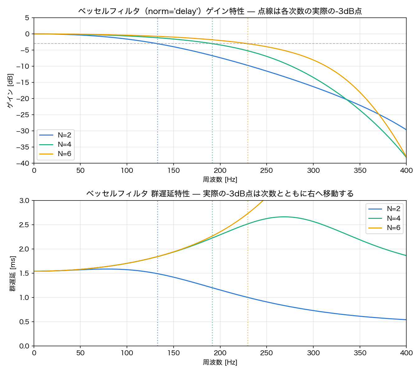
N=2: actual -3dB frequency=132.57 Hz  (nominal fc=100 Hz)
N=4: actual -3dB frequency=191.59 Hz  (nominal fc=100 Hz)
N=6: actual -3dB frequency=229.43 Hz  (nominal fc=100 Hz)
There are two implementation traps hiding here.
Trap 1: the units returned by group_delay(). scipy.signal.group_delay() always returns the group delay gd in samples, even when fs is supplied (fs only rescales the frequency axis w). Treating gd directly as seconds — as an earlier version of this code did — is off by nearly a factor of 1000: this filter’s group delay is only about 1.5–2.7 samples, so plotting it on a 0–0.02 s axis pushes every value off the chart, rendering an empty plot. You must divide by fs (here we also multiply by 1000 for ms) to get real time units.
Trap 2: norm='delay' does not fix the -3dB cutoff. All three filters above are parameterized with fc=100 Hz, yet the actual -3dB frequency is 132.6 Hz for N=2, 191.6 Hz for N=4, and 229.4 Hz for N=6 — drifting further right as the order increases (up to 2.3× the nominal value). That’s because norm='delay' only pins “the group delay value at \(\omega=0\)
”; it leaves the realized passband bandwidth completely unconstrained. The rightward-shifting dotted lines in the figure are the visual proof.
This second trap produces a result that contradicts the intuition “higher order should mean flatter group delay.” Measured at the single nominal point fc=100 Hz, N=2 gives 1.5704 ms (+2.05% vs. its DC value), N=4 gives 1.7012 ms (+10.55%), and N=6 gives 1.7013 ms (+10.55%) — essentially no improvement from N=4 to N=6. The figure explains why: N=2’s group delay curve has already peaked and started declining by the 100 Hz mark, while N=4 and N=6 are still climbing toward their (much later) peak, because their actual -3dB points sit further out. To compare group delay flatness fairly across orders, you need to normalize against each order’s own realized -3dB cutoff rather than a shared absolute frequency (see “What the norm Parameter Means” below).
Group Delay Comparison with Other Filters
As shown above, norm='delay' does not pin the -3dB cutoff, so comparing filter types fairly requires designing the Bessel filter with norm='mag' (which matches the -3dB cutoff to fc, covered below) so every filter’s realized -3dB cutoff sits at the same 100 Hz:
import numpy as np
import matplotlib.pyplot as plt
from scipy import signal

fs = 1000; fc = 100; N = 4

fig, axes = plt.subplots(2, 1, figsize=(9, 8))

filters = {
    'Bessel': signal.bessel(N, fc, btype='low', fs=fs, norm='mag'),
    'Butterworth': signal.butter(N, fc, btype='low', fs=fs),
    'Chebyshev I (rp=1dB)': signal.cheby1(N, 1.0, fc, btype='low', fs=fs),
    'Elliptic (rp=1,rs=60)': signal.ellip(N, 1.0, 60.0, fc, btype='low', fs=fs),
}

colors = ['#2a78d6', '#1baf7a', '#eda100', '#e34948']

for (name, (b, a)), color in zip(filters.items(), colors):
    w, h = signal.freqz(b, a, worN=4096, fs=fs)
    w_gd, gd = signal.group_delay((b, a), w=4096, fs=fs)
    gd_ms = gd / fs * 1000.0  # samples -> milliseconds

    mask = (w >= 1) & (w <= 90)
    gd_pb = gd_ms[mask]
    print(f"{name:24s}: mean={gd_pb.mean():.3f}ms  min={gd_pb.min():.3f}ms  "
          f"max={gd_pb.max():.3f}ms  spread={(gd_pb.max()-gd_pb.min()):.3f}ms")

    axes[0].plot(w, 20 * np.log10(np.abs(h) + 1e-12), label=name, color=color)
    axes[1].plot(w, gd_ms, label=name, color=color)

axes[0].set_xlim(0, 300); axes[0].set_ylim(-80, 5)
axes[0].set_xlabel('Frequency [Hz]'); axes[0].set_ylabel('Magnitude [dB]')
axes[0].set_title(f'Magnitude Response Comparison (N={N}, -3dB matched at 100Hz)')
axes[0].axvline(fc, color='gray', linestyle='--', alpha=0.5); axes[0].legend(); axes[0].grid(True, alpha=0.3)

axes[1].set_xlim(0, 150); axes[1].set_ylim(0, 12)
axes[1].set_xlabel('Frequency [Hz]'); axes[1].set_ylabel('Group Delay [ms]')
axes[1].set_title(f'Group Delay Comparison (N={N}) — Bessel is flattest')
axes[1].axvline(fc, color='gray', linestyle='--', alpha=0.5); axes[1].legend(); axes[1].grid(True, alpha=0.3)

plt.tight_layout()
plt.savefig('group_delay_comparison.png')
Output (group delay statistics over the 1–90 Hz passband):
Bessel                  : mean=3.340ms  min=3.253ms  max=3.497ms  spread=0.244ms
Butterworth             : mean=4.848ms  min=4.021ms  max=6.522ms  spread=2.501ms
Chebyshev I (rp=1dB)    : mean=5.697ms  min=4.148ms  max=10.450ms  spread=6.302ms
Elliptic (rp=1,rs=60)   : mean=5.539ms  min=3.903ms  max=10.598ms  spread=6.694ms
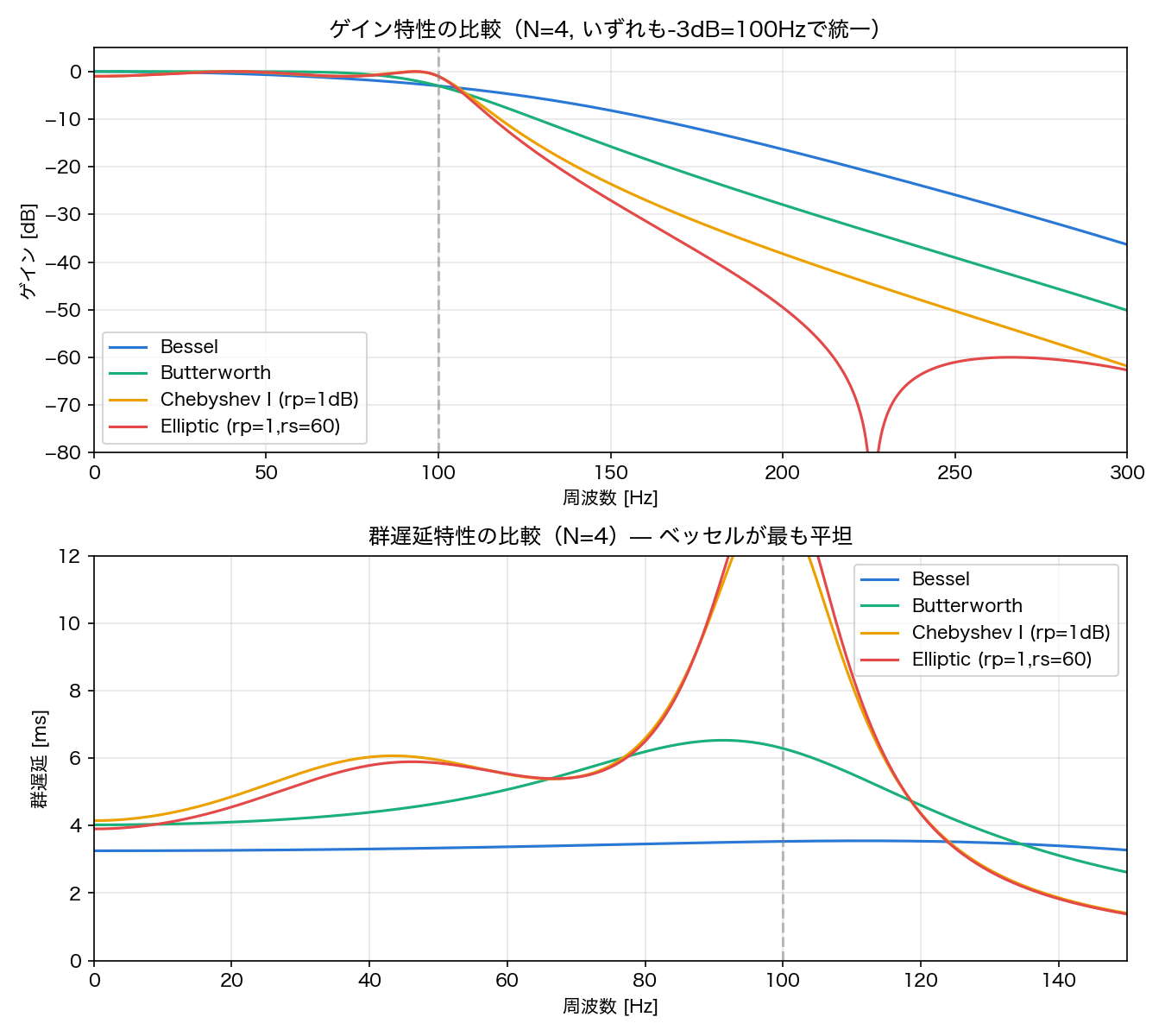
With the -3dB cutoff matched fairly across filter types, Bessel’s group delay spread (0.244 ms) is about 1/10 of Butterworth’s (2.501 ms) and roughly 1/26–1/27 of Chebyshev I’s (6.302 ms) and elliptic’s (6.694 ms). The bottom panel shows the other three filters developing a sharp group-delay peak near the 100 Hz band edge, while the Bessel (blue) curve stays essentially horizontal — direct, measured confirmation of the “maximally flat group delay” design goal.
Pulse Waveform Preservation Example
The following code demonstrates the Bessel filter’s key advantage — preserving rectangular pulse shapes:
import numpy as np
import matplotlib.pyplot as plt
from scipy import signal

fs = 1000; fc = 100; N = 4
t = np.linspace(0, 0.1, int(fs * 0.1), endpoint=False)

# Rectangular pulse (5ms width)
x = np.zeros(len(t))
x[(t >= 0.02) & (t < 0.025)] = 1.0

# As in the previous section, use norm='mag' for Bessel so all four filters
# share the same -3dB cutoff — a fair comparison.
filters = {
    'Bessel': signal.bessel(N, fc, btype='low', fs=fs, norm='mag', output='sos'),
    'Butterworth': signal.butter(N, fc, btype='low', fs=fs, output='sos'),
    'Chebyshev I': signal.cheby1(N, 1.0, fc, btype='low', fs=fs, output='sos'),
    'Elliptic': signal.ellip(N, 1.0, 60.0, fc, btype='low', fs=fs, output='sos'),
}
colors = ['#2a78d6', '#1baf7a', '#eda100', '#e34948']

fig, axes = plt.subplots(len(filters) + 1, 1, figsize=(9, 12), sharex=True)
axes[0].plot(t * 1000, x, 'k', label='Input pulse')
axes[0].set_title('Input Signal (5ms Rectangular Pulse)'); axes[0].legend(); axes[0].grid(True, alpha=0.3)

print(f"{'Filter':12s} {'Peak amp':>10s} {'Peak time[ms]':>14s} {'Delay[ms]':>10s} {'Trailing ringing':>18s}")
for (name, sos), color in zip(filters.items(), colors):
    y = signal.sosfilt(sos, x)

    peak = y.max()
    peak_time = t[np.argmax(y)] * 1000
    delay = peak_time - 22.5  # relative to input pulse center (22.5ms)
    tail_mask = t >= 0.032    # ringing after the pulse's trailing edge
    ringing = np.max(np.abs(y[tail_mask]))
    print(f"{name:12s} {peak:10.4f} {peak_time:14.2f} {delay:10.2f} {ringing:18.4f}")

for idx, ((name, sos), color) in enumerate(zip(filters.items(), colors)):
    y = signal.sosfilt(sos, x)
    ax = axes[idx + 1]
    ax.plot(t * 1000, y, label=name, color=color)
    ax.plot(t * 1000, x, 'k--', alpha=0.3, label='Original pulse')
    ax.set_title(f'{name} (N={N}, -3dB=100Hz)')
    ax.legend(); ax.grid(True, alpha=0.3)

axes[-1].set_xlabel('Time [ms]')
plt.tight_layout()
plt.savefig('pulse_response_comparison.png')
Output:
Filter          Peak amp  Peak time[ms]  Delay[ms]  Trailing ringing
Bessel            0.9396          25.00       2.50             0.0226
Butterworth       0.9433          27.00       4.50             0.1522
Chebyshev I       0.8817          28.00       5.50             0.2285
Elliptic          0.8600          28.00       5.50             0.2473
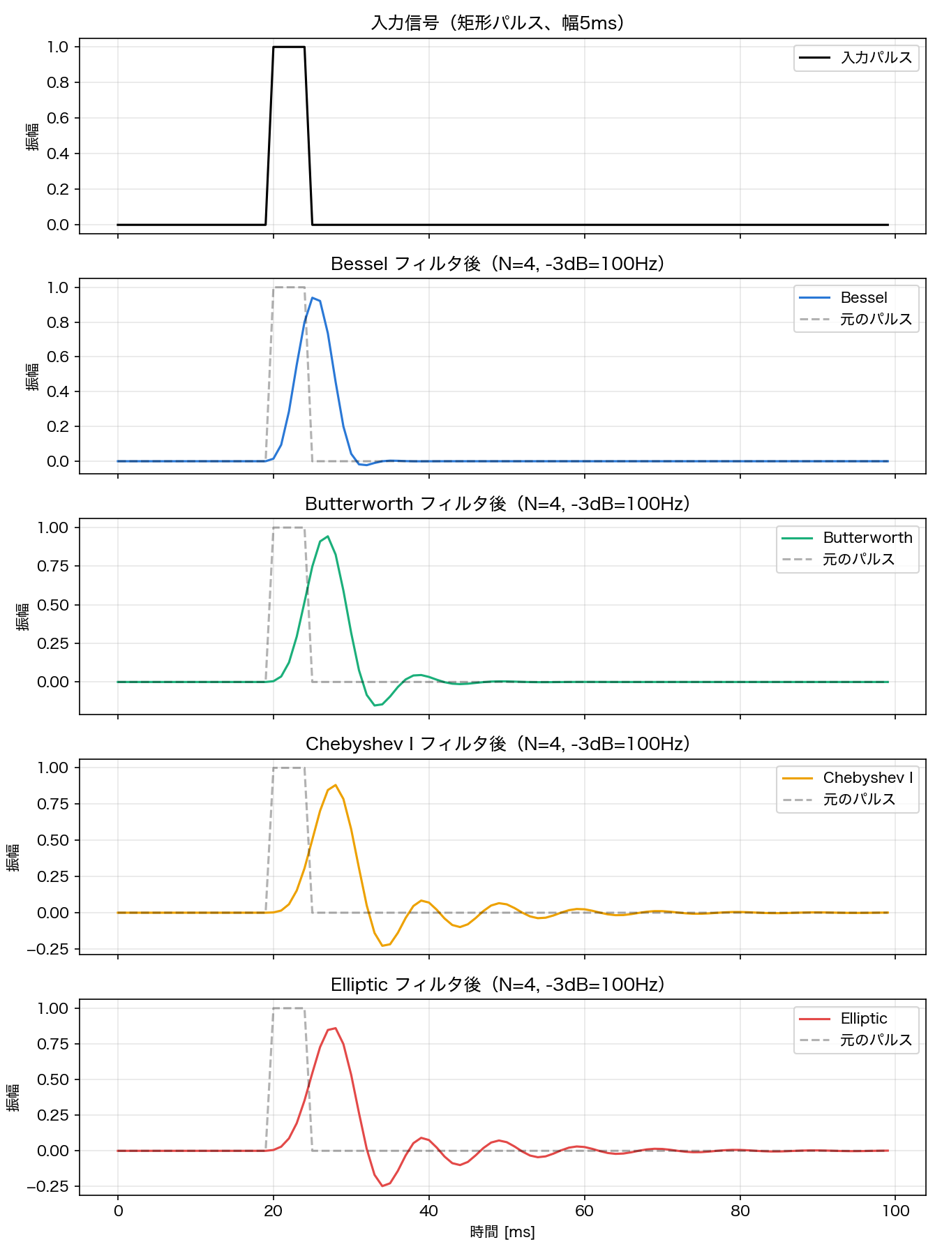
The peak amplitudes themselves are nearly tied — Bessel (0.9396) and Butterworth (0.9433) — because a narrow pulse carries substantial high-frequency content, so every lowpass filter attenuates the peak below 1 regardless of type. What sets Bessel apart is delay and ringing: its peak delay of 2.50 ms is the smallest of the four, and its trailing ringing amplitude of 0.0226 is far below Butterworth’s 0.1522 (about 6.7×) and Chebyshev I/elliptic’s ~0.23 (about 10×). The figure makes this visible directly — only the Bessel (blue) trace decays monotonically after its peak, with no visible oscillation. The Bessel filter’s value isn’t “preserving peak amplitude best” — it’s delaying every frequency component equally and leaving no ringing behind, which is what actually preserves the pulse’s shape.
What the norm Parameter Means
scipy.signal.bessel()’s norm argument selects the normalization convention. Only three values are valid: 'phase', 'delay', and 'mag' — 'critical' does not exist and raises a ValueError if you pass it (verified against SciPy 1.18):
norm value | Meaning | Use Case |
|---|---|---|
'phase' | Phase response reaches its midpoint at angular frequency Wn (default; matches MATLAB’s convention) | Matching Butterworth’s magnitude asymptotes |
'delay' | Group delay at \(\omega=0\) equals \(1/\text{Wn}\) | Evaluating the Bessel filter’s own group delay |
'mag' | Gain equals -3dB at angular frequency Wn | Matching -3dB cutoff against other filter types |
Testing all three at N=4, fc=100 Hz and measuring the actual realized -3dB cutoff:
import numpy as np
from scipy import signal

fs = 1000; fc = 100; N = 4

def find_3db(b, a, fs, fmax=500):
    w = np.linspace(0.01, fmax, 500000)
    _, h = signal.freqz(b, a, worN=w, fs=fs)
    mag_db = 20 * np.log10(np.abs(h) + 1e-300)
    idx = np.argmin(np.abs(mag_db - (-3.0103)))
    return w[idx]

for norm in ['phase', 'delay', 'mag']:
    b, a = signal.bessel(N, fc, btype='low', fs=fs, norm=norm)
    print(f"norm='{norm}': actual -3dB frequency={find_3db(b, a, fs):.2f} Hz")
Output:
norm='phase': actual -3dB frequency=67.28 Hz
norm='delay': actual -3dB frequency=191.57 Hz
norm='mag': actual -3dB frequency=100.00 Hz
Against the nominal fc=100 Hz, the default 'phase' normalization lands at 67.28 Hz (inside the nominal value), while 'delay' lands at 191.57 Hz (outside it, as shown earlier). Only 'mag' hits the specified frequency exactly — and it does so for N=2, 4, and 6 alike (all land at exactly 100.00 Hz), which is why the group delay and pulse-response comparisons above both used norm='mag'. To compare with other filters at a matched -3dB cutoff:
from scipy import signal

fs = 1000; fc = 100; N = 4

# -3dB cutoff at fc=100 Hz
sos_bessel = signal.bessel(N, fc, btype='low', fs=fs, norm='mag', output='sos')
sos_butter = signal.butter(N, fc, btype='low', fs=fs, output='sos')
Conversely, if you want to honor the Bessel filter’s original design intent — pinning the absolute group delay value at \(\omega=0\)
— use norm='delay', but remember from the earlier section that this lets the realized bandwidth widen as the order increases. Whether you should fix the absolute group delay or the -3dB cutoff is the practical question norm answers.
When to Choose a Bessel Filter
| Scenario | Recommended Filter |
|---|---|
| Preserving pulse waveform shape | Bessel filter |
| Minimizing phase distortion in audio signals | Bessel filter |
| Maximizing transition band steepness | Elliptic filter |
| Maximally flat amplitude response in passband | Butterworth filter |
| Minimizing filter order for given spec | Elliptic filter |
| Sharp cutoff with some ripple tolerance | Chebyshev filter |
Recent Research
The Bessel filter’s core property — maximally flat group delay — hasn’t changed since Thomson’s 1952 proposal, but research extending and applying it is still active:
- Kandic, M., & Bridges, G. E. (2025). Maximally Flat Negative Group Delay Prototype Filter Based on Capped Reciprocal Transfer Function of Classical Bessel Filter. Progress In Electromagnetics Research B, 110, 91–105. Takes the ratio of two classical Bessel lowpass transfer functions of the same order but different -3dB bandwidths, producing a prototype with maximally flat negative group delay (the output appears to lead the input rather than lag it) in-band. It reuses the classical Bessel transfer function as a building block for a more elaborate phase response.
- Yi, H., Chang, F., Tan, P., Huang, B., Wu, Y., Xu, Z., Ma, B., & Ma, J. (2025). Design of infinite impulse response maximally flat stable digital filter with low group delay. Scientific Reports, 15, 11074. Proposes a constrained design algorithm for IIR filters that keeps low group delay while preserving stability and magnitude flatness — a numerically-driven alternative to the classical Bessel-polynomial approach, aimed at the same “low group delay, stable IIR” goal.
Both show that the classical goal covered in this article — flattening group delay — is still an active research direction, whether through negative-group-delay circuits or more flexible numerical filter optimization.
Related Articles
- Butterworth Filter Design Principles and Python Implementation - IIR filter with maximally flat passband
- Chebyshev Filter Design Principles and Python Implementation - Equiripple IIR filter design
- Elliptic Filter Design Principles and Python Implementation - Sharpest transition band IIR filter
- FIR vs IIR Filters - Comparison of IIR and FIR design approaches
- Exponential Moving Average (EMA) Filter Frequency Characteristics - EMA as a simple first-order IIR filter
- Lowpass Filter Design and Comparison - Compares moving average, Butterworth, and Chebyshev frequency responses — useful context for Bessel.
- Highpass Filter Design and Python Implementation - Derive the highpass variant from the Bessel LPF prototype for low-frequency drift removal.
- Bandpass Filter Design and Python Implementation - Frequency-transform the Bessel prototype into a bandpass when in-band phase linearity matters.
- Adaptive Filters (LMS/RLS): Theory and Python Implementation - Adaptive counterpart to fixed Bessel design; useful when the channel is non-stationary.
- Bode Plot: Theory and Python Implementation - Bessel’s maximally flat group delay shows up as a near-linear phase plot — the cleanest way to contrast Bessel against Butterworth and Chebyshev.
- Filter Design Selection Guide: 3 axes and characteristic comparison — Use this hub to position the Bessel filter against alternatives during selection.
References
- Thomson, W. E. (1952). Delay networks having maximally flat frequency characteristics. Proceedings of the IEE - Part III: Radio and Communication Engineering, 96(44), 487–490.
- Proakis, J. G., & Manolakis, D. G. (2007). Digital Signal Processing (4th ed.). Pearson.
- SciPy scipy.signal.bessel documentation
- Kandic, M., & Bridges, G. E. (2025). Maximally Flat Negative Group Delay Prototype Filter Based on Capped Reciprocal Transfer Function of Classical Bessel Filter. Progress In Electromagnetics Research B, 110, 91–105. https://www.jpier.org/issues/volume.html?paper=24121308
- Yi, H., Chang, F., Tan, P., Huang, B., Wu, Y., Xu, Z., Ma, B., & Ma, J. (2025). Design of infinite impulse response maximally flat stable digital filter with low group delay. Scientific Reports, 15, 11074. https://www.nature.com/articles/s41598-025-87175-5
Related Tools
- DevToolBox - Free Developer Tools - JSON formatter, regex tester, and 85+ developer utilities
- CalcBox - Everyday Calculators - Statistics, compound interest, and 61+ calculation tools