Introduction
ARIMA has been a classical workhorse for time series forecasting, but it struggles with nonlinear dependencies and long-range patterns. LSTM (Long Short-Term Memory) solves the vanishing gradient problem of vanilla RNNs by introducing a dedicated memory cell, enabling it to capture long-term temporal dependencies.
This article covers the mathematical foundations of LSTM gates and demonstrates practical time series forecasting with PyTorch.
The Limitation of RNNs: Vanishing Gradients
The Hidden-State Recurrence
A standard RNN updates its hidden state as:
\[h_t = \tanh(W_h h_{t-1} + W_x x_t + b) \tag{1}\]Where ordinary neural-network backpropagation is a chain rule that walks backward through depth, backpropagation through time (BPTT) for an RNN is a chain rule that walks backward through time, reusing the same weight matrix \(W_h\) at every step. This section derives, in closed form, the vanishing-gradient phenomenon that is specific to this time-direction recursion.
The Chain Rule Across Time in BPTT
From equation (1), the Jacobian between adjacent hidden states is
\[ \frac{\partial h_t}{\partial h_{t-1}} = \text{diag}\bigl(\tanh'(z_t)\bigr) \, W_h \] \[ \tag{2} \]where \(z_t = W_h h_{t-1} + W_x x_t + b\) (\(\tanh\) acts elementwise, so its Jacobian is diagonal — the same reasoning as in ordinary backprop ).
Differentiating the loss \(L_T\) at time \(T\) with respect to the hidden state \(k\) steps in the past, \(h_{T-k}\) , and applying the chain rule \(k\) times gives
\[ \frac{\partial L_T}{\partial h_{T-k}} = \frac{\partial L_T}{\partial h_T} \prod_{i=T-k+1}^{T} \frac{\partial h_i}{\partial h_{i-1}} = \frac{\partial L_T}{\partial h_T} \prod_{i=T-k+1}^{T} \text{diag}\bigl(\tanh'(z_i)\bigr) \, W_h \] \[ \tag{3} \]Here a product of \(k\) factors of the form “diagonal matrix \(\times\) \(W_h\) ” appears. Unlike depth-wise vanishing gradients in a feedforward network (where each layer typically contributes a different weight matrix once), here the same \(W_h\) is applied \(k\) times in a row — this is the structural difference that is specific to recurrence in time.
Proof of Exponential Decay
Since \(\tanh'(z) = 1-\tanh^2(z) \in (0,1]\) , we have \(\|\text{diag}(\tanh'(z_i))\|_2 \le 1\) . Applying sub-multiplicativity of the operator norm (\(\|AB\|_2 \le \|A\|_2 \|B\|_2\) ) repeatedly to equation (3) gives
\[ \left\| \frac{\partial h_T}{\partial h_{T-k}} \right\|_2 \le \prod_{i=T-k+1}^{T} \|\text{diag}(\tanh'(z_i))\|_2 \, \|W_h\|_2 \le \|W_h\|_2^{\,k} \] \[ \tag{4} \](\(\|W_h\|_2\) is the largest singular value / operator norm of \(W_h\) ; for a symmetric matrix this equals the largest absolute eigenvalue.) Consequently, if \(\|W_h\|_2 < 1\) , the bound in equation (4) decays exponentially to zero as \(k \to \infty\) — this is the precise mathematical content of vanishing gradients. If instead \(\|W_h\|_2 > 1\) , gradients can explode, but because \(\tanh\) saturates, \(\tanh'(z_i)\) shrinks rapidly as \(|z_i|\) grows, so in practice vanishing tends to dominate over exploding (Bengio et al., 1994; Pascanu et al., 2013).
Summing the per-step loss over all time steps, the total gradient is obtained by summing equation (3) over \(t=k,\ldots,T\) :
\[ \frac{\partial L}{\partial h_k} = \sum_{t=k}^{T} \frac{\partial L_t}{\partial h_t} \prod_{i=k+1}^{t} \text{diag}\bigl(\tanh'(z_i)\bigr) \, W_h \] \[ \tag{5} \]By the bound in equation (4), terms with larger \(t-k\) (further away in time) shrink exponentially, so a vanilla RNN has a structural limitation: it can effectively only learn dependencies over the recent past.
LSTM introduces a cell state \(c_t\) — a “memory highway” — that provides an additive path for information flow, separate from the purely multiplicative path of equation (3) (\(\prod \text{diag}(\tanh') W_h\) ). The section “How LSTM Gates Mitigate Vanishing Gradients” below derives this mechanism explicitly.
LSTM Architecture
An LSTM cell has three gates operating on the concatenated input \([h_{t-1}, x_t]\) .
Forget Gate
Decides what information to discard from the previous cell state.
\[f_t = \sigma(W_f [h_{t-1}, x_t] + b_f) \tag{6}\]Values close to 0 mean “forget”; close to 1 mean “keep.”
Input Gate
Controls how much new information to write into the cell state.
\[i_t = \sigma(W_i [h_{t-1}, x_t] + b_i) \tag{7}\] \[\tilde{c}_t = \tanh(W_c [h_{t-1}, x_t] + b_c) \tag{8}\]Cell State Update
Combines the forget and input gates to update the cell state.
\[c_t = f_t \odot c_{t-1} + i_t \odot \tilde{c}_t \tag{9}\]where \(\odot\) denotes the Hadamard (element-wise) product. The additive update preserves gradient flow over long sequences (the mechanism is derived below).
Output Gate
Determines what to expose as the hidden state.
\[o_t = \sigma(W_o [h_{t-1}, x_t] + b_o) \tag{10}\] \[h_t = o_t \odot \tanh(c_t) \tag{11}\]Parameter Count
For input dimension \(d_x\) and hidden dimension \(d_h\) , one LSTM cell has:
\[4 \times (d_h \times (d_x + d_h) + d_h) \tag{12}\]parameters — four weight matrices (\(W_f, W_i, W_c, W_o\) ) each of size \(d_h \times (d_x + d_h)\) plus biases.
Why Three Gates?
Each of the three gates plays an independent role, and removing any one produces a specific, identifiable failure mode.
- Removing the forget gate (fixing \(f_t \equiv 1\) ): the cell update collapses to the plain running sum \(c_t = c_{t-1} + i_t \odot \tilde{c}_t\) . In fact, the original 1997 LSTM (Hochreiter & Schmidhuber, 1997) had exactly this form — no forget gate. Gers, Schmidhuber & Cummins (2000), in “Learning to Forget,” showed that this design causes \(c_t\) to grow without bound on continual (unsegmented) input streams, eventually breaking the network. The forget gate lets the cell actively reset itself at the right moments.
- Removing the input gate (fixing \(i_t \equiv 1\) ): every new candidate \(\tilde{c}_t\) is written into the cell state unconditionally. Noisy or irrelevant inputs pass straight through and corrupt the memory, with no mechanism to filter what is “worth remembering.”
- Removing the output gate (fixing \(o_t \equiv 1\) , so \(h_t = \tanh(c_t)\) ): the full contents of the cell state are exposed as the hidden state at every step. The network loses the ability to keep something in long-term storage while choosing not to expose it as the current-step output.
This intuition is backed by empirical evidence. Greff et al. (2015), in “LSTM: A Search Space Odyssey,” compared eight LSTM variants across three benchmark tasks in roughly 5,400 experimental runs, and found that removing the forget gate or the output activation function (\(\tanh\) ) significantly hurt performance on every task, whereas simplifications such as coupling the input and forget gates (\(i_t = 1-f_t\) , close to a GRU) had little effect. In other words, the three gates are not equally important — the forget gate and the output-side squashing are the two components that matter most.
How LSTM Gates Mitigate Vanishing Gradients
The Direct Partial Derivative of the Cell State
Taking the partial derivative of the cell update in equation (9), \(c_t = f_t \odot c_{t-1} + i_t \odot \tilde{c}_t\) , with respect to \(c_{t-1}\) while treating the gate values \(f_t, i_t, \tilde{c}_t\) as momentarily constant gives
\[ \left. \frac{\partial c_t}{\partial c_{t-1}} \right|_{\text{direct}} = \text{diag}(f_t) \] \[ \tag{13} \]Compare this with the vanilla-RNN Jacobian \(\text{diag}(\tanh'(z_t)) W_h\) from equation (2): there is no linear transform by a weight matrix and no additional \(\tanh'\) attenuation — just the diagonal matrix \(\text{diag}(f_t)\) . As \(f_t \to 1\) (the forget gate fully open), this direct path approaches the identity map \(I\) , and gradients pass through with essentially no decay. This is the mathematical content of what Hochreiter & Schmidhuber (1997) called the “Constant Error Carousel.”
To Be Precise: An Indirect Path Also Exists
\(c_t\) also depends on \(c_{t-1}\) indirectly, through \(h_{t-1}\) (since \(h_{t-1} = o_{t-1} \odot \tanh(c_{t-1})\) , and \(f_t, i_t, \tilde{c}_t\) are all functions of \(h_{t-1}\) ). The full total derivative is
\[ \frac{d c_t}{d c_{t-1}} = \underbrace{\text{diag}(f_t)}_{\text{direct path (eq. 13)}} + \underbrace{\frac{\partial c_t}{\partial h_{t-1}} \cdot \text{diag}(o_{t-1}) \, \text{diag}\bigl(\tanh'(c_{t-1})\bigr)}_{\text{indirect path, via } h_{t-1}} \] \[ \tag{14} \]where \(\partial c_t/\partial h_{t-1}\) contains, for each of \(f_t, i_t, \tilde{c}_t\) , a product of a sigmoid/\(\tanh\) derivative with the corresponding weight matrix \(W_f, W_i, W_c\) . In other words, the indirect path has exactly the same multiplicative structure as a vanilla RNN, and can vanish on its own. This is precisely why LSTM is said to mitigate, not solve, vanishing gradients.
Even so, the direct path in equation (13) exists independently of the indirect one, and extracting only the \(k\) -step direct path gives
\[ \frac{\partial c_t}{\partial c_{t-k}} \supseteq \prod_{i=t-k+1}^{t} \text{diag}(f_i) \] \[ \tag{15} \]which is always present additively. Unlike the vanilla-RNN bound \(\|W_h\|_2^{\,k}\) from equation (4), this term contains no weight matrix at all, and as long as \(f_i \approx 1\) it does not decay appreciably even as \(k\) grows. So over any stretch of time where the forget gate has learned (or been initialized) to stay close to 1, the gradient flowing through the cell state is preserved additively over long horizons.
An important caveat: this mitigating effect is conditional on \(f_t \approx 1\)
. Since \(f_t\)
is a learned quantity, without any special initialization it starts out around \(f_t \approx 0.5\)
(see the numerical experiment below), and the direct path in equation (15) then decays on the order of \(0.5^k\)
— essentially no better than a vanilla RNN. A well-known practical fix is due to Jozefowicz et al. (2015), who recommend initializing the forget-gate bias \(b_f\)
to a positive value around 1; this trick is applied manually in many LSTM implementations (including on top of PyTorch’s nn.LSTM). We measure its effect directly in the next section.
Empirical Verification: Gradient Norms in RNN vs. LSTM
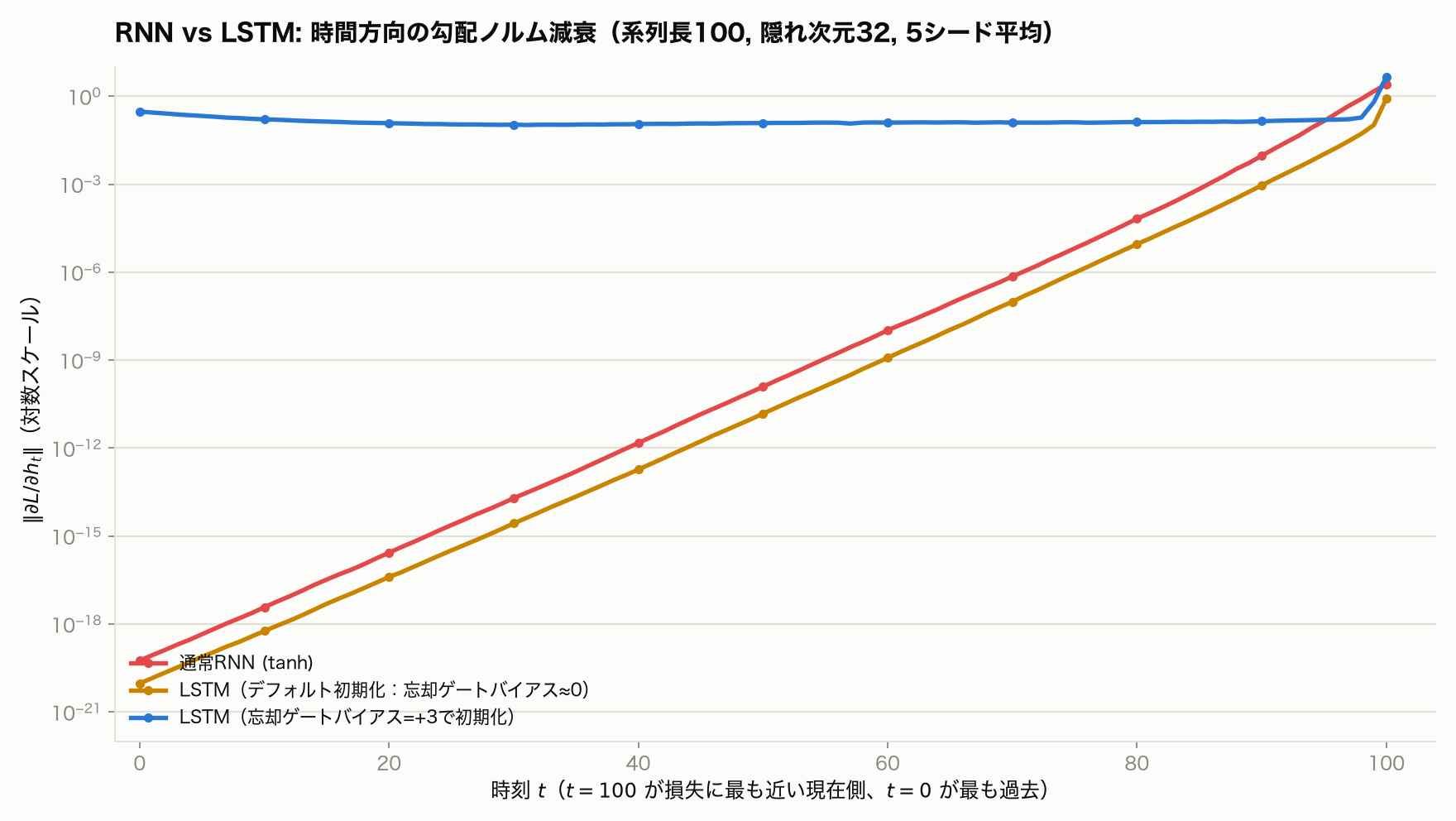
To see how large the theoretical mitigation effect actually is, we measure it directly in PyTorch. For a sequence length of 100 and hidden size 32, we compare (1) a vanilla RNN (tanh), (2) an LSTM with default initialization, and (3) an LSTM whose forget-gate bias is initialized to \(+3\) . For each, we compute the gradient norm \(\|\partial L/\partial h_t\|\) from the final-step loss \(L = \|h_{100}\|^2\) back to the hidden state at every time step \(t\) .
import numpy as np
import torch
import torch.nn as nn

SEQ_LEN = 100
INPUT_SIZE = 1
HIDDEN_SIZE = 32
N_TRIALS = 5  # average over several seeds to smooth out init-dependent noise


def run_rnn_trial(seed):
    torch.manual_seed(seed)
    rnn = nn.RNN(input_size=INPUT_SIZE, hidden_size=HIDDEN_SIZE,
                 nonlinearity="tanh", batch_first=True)
    Wx, Wh, bx, bh = rnn.weight_ih_l0, rnn.weight_hh_l0, rnn.bias_ih_l0, rnn.bias_hh_l0

    x = torch.randn(SEQ_LEN, INPUT_SIZE)
    h_list = [torch.zeros(1, HIDDEN_SIZE, requires_grad=True)]
    for t in range(SEQ_LEN):
        h_prev = h_list[-1]
        h_prev.retain_grad()
        z = x[t:t+1] @ Wx.T + bx + h_prev @ Wh.T + bh
        h_list.append(torch.tanh(z))
    h_list[-1].retain_grad()
    loss = h_list[-1].pow(2).sum()
    loss.backward()
    return np.array([0.0 if h.grad is None else h.grad.norm().item() for h in h_list])


def run_lstm_trial(seed, forget_bias_init=None):
    torch.manual_seed(seed)
    lstm = nn.LSTM(input_size=INPUT_SIZE, hidden_size=HIDDEN_SIZE, batch_first=True)
    H = HIDDEN_SIZE
    Wi, Wh_l, bi, bh_l = lstm.weight_ih_l0, lstm.weight_hh_l0, lstm.bias_ih_l0, lstm.bias_hh_l0

    if forget_bias_init is not None:
        with torch.no_grad():
            bi[H:2*H] = forget_bias_init / 2
            bh_l[H:2*H] = forget_bias_init / 2  # PyTorch gate order is [i, f, g, o]

    x = torch.randn(SEQ_LEN, INPUT_SIZE)

    def cell(x_t, h_prev, c_prev):
        gates = x_t @ Wi.T + bi + h_prev @ Wh_l.T + bh_l
        i_g = torch.sigmoid(gates[:, 0:H])
        f_g = torch.sigmoid(gates[:, H:2*H])
        g_g = torch.tanh(gates[:, 2*H:3*H])
        o_g = torch.sigmoid(gates[:, 3*H:4*H])
        c_new = f_g * c_prev + i_g * g_g
        h_new = o_g * torch.tanh(c_new)
        return h_new, c_new

    h_list = [torch.zeros(1, H, requires_grad=True)]
    c_list = [torch.zeros(1, H, requires_grad=True)]
    for t in range(SEQ_LEN):
        h_prev, c_prev = h_list[-1], c_list[-1]
        h_prev.retain_grad()
        c_prev.retain_grad()
        h_new, c_new = cell(x[t:t+1], h_prev, c_prev)
        h_list.append(h_new)
        c_list.append(c_new)
    h_list[-1].retain_grad()
    loss = h_list[-1].pow(2).sum()
    loss.backward()
    return np.array([0.0 if h.grad is None else h.grad.norm().item() for h in h_list])


rnn_curves = np.stack([run_rnn_trial(s) for s in range(N_TRIALS)])
lstm_default_curves = np.stack([run_lstm_trial(s, forget_bias_init=None) for s in range(N_TRIALS)])
lstm_biased_curves = np.stack([run_lstm_trial(s, forget_bias_init=3.0) for s in range(N_TRIALS)])

rnn_mean = rnn_curves.mean(axis=0)
lstm_default_mean = lstm_default_curves.mean(axis=0)
lstm_biased_mean = lstm_biased_curves.mean(axis=0)
The results (averaged over 5 seeds; \(t=100\) is the step closest to the loss, \(t=0\) is furthest in the past) are:
| \(t\) | Vanilla RNN (tanh) | LSTM (default init) | LSTM (forget bias \(+3\) ) |
|---|---|---|---|
| 0 | \(5.68 \times 10^{-20}\) | \(9.47 \times 10^{-21}\) | \(3.01 \times 10^{-1}\) |
| 30 | \(1.97 \times 10^{-14}\) | \(2.70 \times 10^{-15}\) | \(1.08 \times 10^{-1}\) |
| 50 | \(1.25 \times 10^{-10}\) | \(1.50 \times 10^{-11}\) | \(1.22 \times 10^{-1}\) |
| 70 | \(7.15 \times 10^{-7}\) | \(9.79 \times 10^{-8}\) | \(1.26 \times 10^{-1}\) |
| 90 | \(9.36 \times 10^{-3}\) | \(9.14 \times 10^{-4}\) | \(1.41 \times 10^{-1}\) |
| 100 | \(2.57\) | \(8.22 \times 10^{-1}\) | \(4.58\) |
Taking the ratio of \(t=0\) to \(t=100\) (a rough measure of gradient preservation over 100 steps): the vanilla RNN gives \(2.22 \times 10^{-20}\) , and the default-initialized LSTM gives \(1.15 \times 10^{-20}\) — essentially the same order of magnitude as the vanilla RNN. The LSTM with forget bias initialized to \(+3\) gives \(6.57 \times 10^{-2}\) — nearly 18 orders of magnitude more gradient preserved.
This matches the theory in equations (13)–(15) exactly. Since \(\sigma(0)=0.5\) , under default initialization (bias \(\approx 0\) ) the forget gate averages around \(f_t \approx 0.5\) , so the direct path in equation (15) also decays on the order of \(0.5^{100}\) — essentially no different from the vanilla RNN. Since \(\sigma(3.0) \approx 0.953\) , initializing the forget bias to \(+3\) pushes \(f_t \approx 0.95\) , so the direct path stays around \(0.95^{100} \approx 6 \times 10^{-3}\) and dominates, preserving the gradient. “LSTM automatically solves vanishing gradients” is not quite right — the mitigation only kicks in once the forget gate is actually close to 1, and this is the single most important caveat of this section.
LSTM for Time Series Forecasting
The standard Seq2One setup feeds a window of \(T\) past values \(\{x_{t-T+1}, \ldots, x_t\}\) and predicts \(x_{t+1}\) .
| Setup | Input | Output | Use Case |
|---|---|---|---|
| Seq2One | sequence → 1 | single-step | Next-step prediction |
| Seq2Seq | sequence → seq | multi-step | Multi-horizon forecast |
| Encoder-Decoder | variable-length | variable-length | Translation, anomaly |
Python Implementation (PyTorch)
Data Preparation
We use a noisy sine wave as a synthetic time series.
import numpy as np
import torch
import torch.nn as nn
from torch.utils.data import DataLoader, TensorDataset
import matplotlib.pyplot as plt

# Synthetic time series
np.random.seed(42)
t = np.linspace(0, 8 * np.pi, 1000)
data = np.sin(t) + 0.2 * np.random.randn(len(t))

# Normalize
data_mean, data_std = data.mean(), data.std()
data_norm = (data - data_mean) / data_std

def create_sequences(data, seq_len):
    X, y = [], []
    for i in range(len(data) - seq_len):
        X.append(data[i:i + seq_len])
        y.append(data[i + seq_len])
    return np.array(X), np.array(y)

SEQ_LEN = 30
X, y = create_sequences(data_norm, SEQ_LEN)

split = int(len(X) * 0.8)
X_train, X_test = X[:split], X[split:]
y_train, y_test = y[:split], y[split:]

# Shape: [batch, seq_len, features]
X_train_t = torch.FloatTensor(X_train).unsqueeze(-1)
X_test_t  = torch.FloatTensor(X_test).unsqueeze(-1)
y_train_t = torch.FloatTensor(y_train).unsqueeze(-1)
y_test_t  = torch.FloatTensor(y_test).unsqueeze(-1)

train_loader = DataLoader(
    TensorDataset(X_train_t, y_train_t),
    batch_size=32, shuffle=True
)
Model Definition
class LSTMForecaster(nn.Module):
    def __init__(self, input_size=1, hidden_size=64, num_layers=2, dropout=0.2):
        super().__init__()
        self.lstm = nn.LSTM(
            input_size=input_size,
            hidden_size=hidden_size,
            num_layers=num_layers,
            batch_first=True,
            dropout=dropout if num_layers > 1 else 0.0
        )
        self.fc = nn.Linear(hidden_size, 1)

    def forward(self, x):
        out, _ = self.lstm(x)
        return self.fc(out[:, -1, :])  # last timestep

model = LSTMForecaster(hidden_size=64, num_layers=2)
criterion = nn.MSELoss()
optimizer = torch.optim.Adam(model.parameters(), lr=1e-3)
Training Loop
EPOCHS = 50
train_losses = []

for epoch in range(EPOCHS):
    model.train()
    epoch_loss = 0.0
    for X_batch, y_batch in train_loader:
        optimizer.zero_grad()
        pred = model(X_batch)
        loss = criterion(pred, y_batch)
        loss.backward()
        nn.utils.clip_grad_norm_(model.parameters(), max_norm=1.0)
        optimizer.step()
        epoch_loss += loss.item()
    train_losses.append(epoch_loss / len(train_loader))

    if (epoch + 1) % 10 == 0:
        print(f"Epoch {epoch+1}/{EPOCHS}  Loss: {train_losses[-1]:.6f}")
Prediction and Evaluation
model.eval()
with torch.no_grad():
    pred_norm = model(X_test_t).numpy().squeeze()

pred = pred_norm * data_std + data_mean
true = y_test * data_std + data_mean

rmse = np.sqrt(np.mean((pred - true) ** 2))
print(f"RMSE: {rmse:.4f}")

plt.figure(figsize=(12, 4))
plt.plot(true, label="Ground Truth", alpha=0.7)
plt.plot(pred, label="LSTM Prediction", alpha=0.7)
plt.xlabel("Time Step")
plt.ylabel("Value")
plt.title("LSTM Time Series Forecasting")
plt.legend()
plt.grid(True)
plt.tight_layout()
plt.show()
Running this code actually produces a RMSE \(\approx 0.2115\) on the test set (random seed 42, original scale).
ARIMA vs LSTM Comparison
| Aspect | ARIMA | LSTM |
|---|---|---|
| Stationarity | Required (differencing helps) | Not required |
| Nonlinearity | No | Yes |
| Long-range deps | Weak (low-order ARIMA) | Strong (cell state) |
| Parameter count | Few (p, d, q) | Many (thousands) |
| Interpretability | High (coefficient meaning) | Low (black box) |
| Data requirement | Small datasets OK | Needs substantial data |
| Training speed | Fast | Slow (GPU accelerates) |
| Overfitting risk | Low | High (Dropout mitigates) |
Decision guide:
- Small data, linear seasonality → ARIMA/SARIMA
- Nonlinear patterns, multivariate, large data → LSTM
- Real-time inference required → Lightweight LSTM or ARIMA
Measuring Forecast Accuracy Under a Fair Comparison
We fit
ARIMA
(2,1,0) on the same synthetic data as the LSTM above (noisy sine wave, SEQ_LEN=30, 80/20 split) to compare them directly.
from statsmodels.tsa.arima.model import ARIMA

raw_train = data[:split + SEQ_LEN]
raw_test = data[split + SEQ_LEN:]

# (a) Dynamic multi-step forecast: never sees the true test values
model = ARIMA(raw_train, order=(2, 1, 0))
fit = model.fit()
multi_step_pred = fit.forecast(steps=len(raw_test))
rmse_multistep = np.sqrt(np.mean((multi_step_pred - raw_test) ** 2))

# (b) One-step walk-forward: sees the true value up to the previous step
# (same condition as the LSTM's Seq2One: the previous SEQ_LEN true values are known)
history_fit = fit
one_step_preds = []
for i in range(len(raw_test)):
    pred = history_fit.forecast(steps=1)[0]
    one_step_preds.append(pred)
    history_fit = history_fit.append([raw_test[i]], refit=False)
rmse_onestep = np.sqrt(np.mean((np.array(one_step_preds) - raw_test) ** 2))
The results:
| Method | RMSE | Condition |
|---|---|---|
| LSTM (Seq2One) | \(0.2115\) | Previous 30 true values known, predicts 1 step ahead |
| ARIMA(2,1,0) dynamic multi-step | \(1.2796\) | Pure extrapolation past the training set, never sees test data |
| ARIMA(2,1,0) one-step walk-forward | \(0.2245\) | True value known up to the previous step (same condition as LSTM) |
This comparison comes with an important caveat. Looking only at “LSTM RMSE \(0.21\)
vs. ARIMA dynamic-forecast RMSE \(1.28\)
” makes it look like LSTM beats ARIMA by nearly 6×, but the conditions are not comparable. The LSTM’s Seq2One setup always sees the true previous 30 values and only predicts 1 step ahead, whereas ARIMA’s forecast(steps=len(raw_test)) extrapolates the entire test horizon without ever consulting the true test values, which lets phase errors accumulate on a periodic series. Running ARIMA under the same “true history known, predict 1 step ahead” condition (walk-forward, code block (b) above) improves its RMSE to \(0.2245\)
— essentially tied with LSTM’s \(0.2115\)
. For a single-series, one-step-ahead forecasting task on a simple sine wave, LSTM’s nonlinear representational power provides limited advantage, and ARIMA alone is already competitive. LSTM’s real value shows up when nonlinearity is strong, the series is multivariate, or long-range dependence genuinely matters.
Multivariate Extension
To use multiple input features, simply change input_size:
# Example: predict temperature from [temp, humidity, pressure]
model = LSTMForecaster(input_size=3, hidden_size=128, num_layers=2)
# X_train_t: [batch, seq_len, 3]
Measuring the Effect of Multivariate Inputs
We generate a synthetic 3-variable series mimicking temperature, humidity, and pressure (sine waves at different periods and phases plus noise, 1000 time steps), and compare (a) an LSTM using all three variables to predict the next temperature value against (b) an LSTM using only the univariate temperature series, under identical training settings (hidden_size=64, num_layers=2, epochs=50, reusing the same LSTMForecaster class from the “Model Definition” section above).
np.random.seed(7)
n = 1000
time = np.linspace(0, 8 * np.pi, n)
temp = 20 + 5 * np.sin(time) + 0.3 * np.random.randn(n)
humidity = 60 - 10 * np.sin(time + 0.5) + 0.5 * np.random.randn(n)
pressure = 1013 + 3 * np.sin(time * 0.5) + 0.2 * np.random.randn(n)

mv_data = np.stack([temp, humidity, pressure], axis=1)  # [n, 3]
mv_mean, mv_std = mv_data.mean(axis=0), mv_data.std(axis=0)
mv_norm = (mv_data - mv_mean) / mv_std

def create_mv_sequences(data, seq_len):
    X, y = [], []
    for i in range(len(data) - seq_len):
        X.append(data[i:i + seq_len, :])   # [seq_len, 3]
        y.append(data[i + seq_len, 0])     # predict next temperature (column 0) only
    return np.array(X), np.array(y)

MV_SEQ_LEN = 30
Xm, ym = create_mv_sequences(mv_norm, MV_SEQ_LEN)
mv_split = int(len(Xm) * 0.8)
Xm_train_t = torch.FloatTensor(Xm[:mv_split])
Xm_test_t  = torch.FloatTensor(Xm[mv_split:])
ym_train_t = torch.FloatTensor(ym[:mv_split]).unsqueeze(-1)
ym_test_t  = torch.FloatTensor(ym[mv_split:]).unsqueeze(-1)

mv_loader = DataLoader(TensorDataset(Xm_train_t, ym_train_t), batch_size=32, shuffle=True)

# (a) All three variables as input (LSTMForecaster reused from "Model Definition")
mv_model = LSTMForecaster(input_size=3, hidden_size=64, num_layers=2)
mv_optimizer = torch.optim.Adam(mv_model.parameters(), lr=1e-3)
for epoch in range(EPOCHS):
    mv_model.train()
    for Xb, yb in mv_loader:
        mv_optimizer.zero_grad()
        loss = criterion(mv_model(Xb), yb)
        loss.backward()
        nn.utils.clip_grad_norm_(mv_model.parameters(), max_norm=1.0)
        mv_optimizer.step()

mv_model.eval()
with torch.no_grad():
    mv_pred = mv_model(Xm_test_t).numpy().squeeze() * mv_std[0] + mv_mean[0]
mv_true = ym[mv_split:] * mv_std[0] + mv_mean[0]
rmse_mv = np.sqrt(np.mean((mv_pred - mv_true) ** 2))

# (b) Baseline: univariate temperature only (same series, same split, same training)
temp_norm = (temp - temp.mean()) / temp.std()
Xu, yu = create_sequences(temp_norm, MV_SEQ_LEN)   # create_sequences is the same helper from "Data Preparation"
Xu_train_t = torch.FloatTensor(Xu[:mv_split]).unsqueeze(-1)
Xu_test_t  = torch.FloatTensor(Xu[mv_split:]).unsqueeze(-1)
yu_train_t = torch.FloatTensor(yu[:mv_split]).unsqueeze(-1)
u_loader = DataLoader(TensorDataset(Xu_train_t, yu_train_t), batch_size=32, shuffle=True)

u_model = LSTMForecaster(input_size=1, hidden_size=64, num_layers=2)
u_optimizer = torch.optim.Adam(u_model.parameters(), lr=1e-3)
for epoch in range(EPOCHS):
    u_model.train()
    for Xb, yb in u_loader:
        u_optimizer.zero_grad()
        loss = criterion(u_model(Xb), yb)
        loss.backward()
        nn.utils.clip_grad_norm_(u_model.parameters(), max_norm=1.0)
        u_optimizer.step()

u_model.eval()
with torch.no_grad():
    u_pred = u_model(Xu_test_t).numpy().squeeze() * temp.std() + temp.mean()
u_true = yu[mv_split:] * temp.std() + temp.mean()
rmse_uni = np.sqrt(np.mean((u_pred - u_true) ** 2))

print(f"Multivariate LSTM RMSE: {rmse_mv:.4f}   Univariate LSTM RMSE: {rmse_uni:.4f}")
The result: the 3-variable LSTM achieves RMSE \(0.2948\) , while the temperature-only LSTM achieves RMSE \(0.3188\) — a roughly 7.5% improvement from adding the extra variables. Humidity and pressure carry genuinely useful information for predicting temperature here (this improvement depends on how correlated the extra variables actually are — adding unrelated variables would not help).
Recent Research Trends (2023 Onward): Where LSTM Stands Today
The era when LSTM was the default choice for time series forecasting has passed; since around 2023 the field’s center of gravity has shifted decisively toward Transformer-based, linear, and state-space model architectures. Here is a brief overview of the main threads, followed by an honest assessment of where LSTM stands today.
- DLinear (the revenge of linear models): Zeng et al. (2023), “Are Transformers Effective for Time Series Forecasting?” (AAAI 2023), showed that DLinear — decomposing a series into trend and seasonal components and fitting each with a simple linear layer — outperforms many contemporaneous Transformer-based SOTA models, sparking considerable debate. The paper raises the question of whether Self-Attention’s permutation-invariance is actually at odds with the strong inductive bias of temporal order, and it renewed appreciation for testing a simple linear baseline before reaching for a complex architecture.
- PatchTST: Nie et al. (2023, ICLR), “A Time Series is Worth 64 Words,” splits a series into patches (sub-windows) that serve as Transformer tokens, and combines this with channel independence (processing each variate separately) to substantially improve long-horizon accuracy.
- iTransformer: Liu et al. (2024, ICLR) propose an “inverted” Transformer that tokenizes along the variate axis instead of the time axis, letting attention directly capture cross-variate correlations in multivariate series, and report strong results.
- TimesNet: Wu et al. (2023, ICLR) fold a 1D time series into 2D tensors based on detected periodicities, then apply an Inception-style block (borrowed from vision architectures) to model multiple periods simultaneously.
- Mamba-based state space models: Gu & Dao’s (2023–2024) Mamba (a Selective State Space Model) preserves the sequential, RNN-like inductive bias for updating state while achieving Transformer-level training efficiency through a hardware-aware parallel scan algorithm. Several 2024 papers (e.g., MambaTS, TimeMachine) adapt Mamba specifically to time series forecasting. Its linear time and memory complexity for long sequences is, in spirit, a direct descendant of the RNN/LSTM lineage.
These developments are covered in more depth in Transformer for Time Series Forecasting . Being honest about where LSTM stands today: on large-scale, multivariate, long-horizon public benchmarks it is now routinely outperformed by the architectures above. That said, LSTM retains real practical value for several reasons: (1) it is a lightweight baseline with far fewer parameters and FLOPs, training quickly; (2) its gate activations offer at least some traceable structure, arguably more of a foothold for interpretation than a multi-head attention map; (3) as our own measurement above showed, on univariate, short-to-medium-horizon tasks it often ties with classical methods like ARIMA, so reaching for an overly complex model is not always warranted; and (4) it suits streaming inference well, since each step updates its state in constant time and constant memory, unlike a Transformer that must reprocess (or cache) the whole input window. For all these reasons, LSTM remains a solid “lightweight nonlinear baseline to try first.”
Related Articles
- Time Series Forecasting Fundamentals: ARIMA Theory and Python Implementation — classical linear forecasting method; compare interpretability vs LSTM.
- PACF and AR Model Order Identification — identifying the classical AR order with the PACF; also a statistically grounded hint for choosing the LSTM lookback (input sequence length).
- Self-Attention Theory and Python Implementation — the attention mechanism that succeeded LSTM in sequence modeling.
- Transformer for Time Series Forecasting — a deeper dive into PatchTST, Informer, and Autoformer, the lineage of long-horizon models that succeeded LSTM.
- SGD and Adam Optimizer Theory and Python Implementation — details on the Adam optimizer used to train LSTM.
- Time Series Anomaly Detection: From Statistical Methods to Kalman Filters — anomaly detection approaches applicable alongside LSTM forecasting; the LSTM residual itself is a natural anomaly score.
- Machine Learning Hub for Time-Series, Classification, and Anomaly Detection — Hub article placing LSTM among seven methods (k-means/GMM, RF/GBDT, LSTM, Kalman, Isolation Forest) across three selection axes and nine decision scenarios.
- Ensemble Learning: From Decision Trees to Random Forest and Gradient Boosting — GBDT-with-lag-features vs LSTM is the canonical baseline contrast; GBDT often wins on short-to-medium horizons.
- Bayesian Optimization: Fundamentals and Python Implementation
— Automatic search of LSTM
hidden_size / layers / lookback / learning_ratein 20–50 trials with TPE or GP-EI in Optuna.
References
- Hochreiter, S., & Schmidhuber, J. (1997). Long Short-Term Memory. Neural Computation, 9(8), 1735–1780.
- Gers, F. A., Schmidhuber, J., & Cummins, F. (2000). Learning to Forget: Continual Prediction with LSTM. Neural Computation, 12(10), 2451–2471.
- Greff, K., Srivastava, R. K., Koutník, J., Steunebrink, B. R., & Schmidhuber, J. (2015). LSTM: A Search Space Odyssey. arXiv:1503.04069.
- Jozefowicz, R., Zaremba, W., & Sutskever, I. (2015). An Empirical Exploration of Recurrent Network Architectures. ICML 2015.
- Bengio, Y., Simard, P., & Frasconi, P. (1994). Learning Long-Term Dependencies with Gradient Descent is Difficult. IEEE Transactions on Neural Networks, 5(2), 157–166.
- Pascanu, R., Mikolov, T., & Bengio, Y. (2013). On the Difficulty of Training Recurrent Neural Networks. ICML 2013.
- Zeng, A., Chen, M., Zhang, L., & Xu, Q. (2023). Are Transformers Effective for Time Series Forecasting? AAAI 2023.
- Nie, Y., Nguyen, N. H., Sinthong, P., & Kalagnanam, J. (2023). A Time Series is Worth 64 Words: Long-term Forecasting with Transformers. ICLR 2023.
- Liu, Y., Hu, T., Zhang, H., Wu, H., Wang, S., Ma, L., & Long, M. (2024). iTransformer: Inverted Transformers Are Effective for Time Series Forecasting. ICLR 2024.
- Wu, H., Hu, T., Liu, Y., Zhou, H., Wang, J., & Long, M. (2023). TimesNet: Temporal 2D-Variation Modeling for General Time Series Analysis. ICLR 2023.
- Gu, A., & Dao, T. (2023). Mamba: Linear-Time Sequence Modeling with Selective State Spaces. arXiv:2312.00752.
- PyTorch Documentation: torch.nn.LSTM
Related Tools
- DevToolBox - Free Developer Tools - JSON formatter, regex tester, and 85+ developer tools
- CalcBox - Everyday Calculators - Statistics, compound interest, and 61+ calculators