Introduction
When analyzing audio, vibration, or biomedical signals, it is often necessary to know the instantaneous amplitude or instantaneous frequency at each point in time. However, the conventional Fourier transform only reveals the overall frequency content of a signal, losing the information about when each frequency component is present.
The Hilbert Transform is a powerful tool that solves this problem. By using the Hilbert transform to construct the Analytic Signal, we can directly compute the instantaneous amplitude, instantaneous phase, and instantaneous frequency of any real signal.
This article covers the mathematical definition of the Hilbert transform through to practical Python implementations using scipy.signal.hilbert.
Definition of the Hilbert Transform
Continuous-Time Hilbert Transform
The Hilbert transform \(\hat{x}(t)\) of a real signal \(x(t)\) is defined as:
\[\hat{x}(t) = \mathcal{H}\{x(t)\} = \frac{1}{\pi} \text{P.V.} \int_{-\infty}^{\infty} \frac{x(\tau)}{t - \tau} d\tau \tag{1}\]where P.V. denotes the Cauchy principal value integral, which symmetrically avoids the singularity at \(t = \tau\) .
Equation \((1)\) can be viewed as the convolution of \(x(t)\) with \(h(t) = \frac{1}{\pi t}\) :
\[\hat{x}(t) = x(t) * \frac{1}{\pi t} \tag{2}\]Frequency-Domain Interpretation
By the convolution theorem, the Hilbert transform takes a particularly elegant form in the frequency domain:
\[\hat{X}(f) = H(f) \cdot X(f) \tag{3}\]where the filter \(H(f)\) is:
\[H(f) = \begin{cases} -j & (f > 0) \\ 0 & (f = 0) \\ +j & (f < 0) \end{cases} \tag{4}\]In other words, the Hilbert transform is an all-pass filter that shifts positive frequency components by \(-90°\) and negative frequency components by \(+90°\) . The amplitude spectrum is unchanged; only the phase is rotated.
This property leads to the well-known result: applying the Hilbert transform to a cosine gives a sine:
\[\mathcal{H}\{\cos(2\pi f_0 t)\} = \sin(2\pi f_0 t) \tag{5}\]Analytic Signal
Definition
From a real signal \(x(t)\) , we construct the analytic signal \(z(t)\) as:
\[z(t) = x(t) + j\hat{x}(t) \tag{6}\]The analytic signal is complex-valued: its real part is the original signal \(x(t)\) and its imaginary part is the Hilbert transform \(\hat{x}(t)\) .
In the frequency domain:
\[Z(f) = \begin{cases} 2X(f) & (f > 0) \\ X(0) & (f = 0) \\ 0 & (f < 0) \end{cases} \tag{7}\]That is, the analytic signal suppresses the negative-frequency components and doubles the positive-frequency components. This one-sided spectrum representation is what makes instantaneous feature extraction possible.
Instantaneous Amplitude, Phase, and Frequency
Writing the analytic signal in polar form:
\[z(t) = A(t) \cdot e^{j\phi(t)} \tag{8}\]we can directly extract the following instantaneous characteristics.
Instantaneous amplitude (envelope):
\[A(t) = |z(t)| = \sqrt{x(t)^2 + \hat{x}(t)^2} \tag{9}\]Instantaneous phase:
\[\phi(t) = \angle z(t) = \arctan\!\left(\frac{\hat{x}(t)}{x(t)}\right) \tag{10}\]Instantaneous frequency:
\[f_i(t) = \frac{1}{2\pi} \frac{d\phi(t)}{dt} \tag{11}\]The instantaneous frequency is the time derivative of the phase and tracks how the signal’s frequency evolves over time.
Python Implementation
Using scipy.signal.hilbert
SciPy provides scipy.signal.hilbert, which computes the analytic signal efficiently:
from scipy.signal import hilbert
import numpy as np

# Input signal
x = np.array([...])  # real-valued signal

# Compute the analytic signal (uses discrete Hilbert transform internally)
z = hilbert(x)

# Instantaneous amplitude (envelope)
amplitude = np.abs(z)

# Instantaneous phase (radians)
phase = np.angle(z)

# Instantaneous frequency (Hz)
fs = 1000  # sampling frequency
inst_freq = np.diff(np.unwrap(phase)) / (2 * np.pi) * fs
scipy.signal.hilbert is implemented using the FFT, with complexity \(O(N \log N)\)
. Internally it applies the frequency-domain filter in equation \((4)\)
and returns the analytic signal \(z(t)\)
.
Note: The return value of
scipy.signal.hilbertis the full analytic signal \(z(t)\) (real part = original signal, imaginary part = Hilbert transform). To obtain only \(\hat{x}(t)\) , usenp.imag(hilbert(x)).
Basic Verification
We verify the \(\mathcal{H}\{\cos\} = \sin\) identity numerically:
import numpy as np
import matplotlib.pyplot as plt
from scipy.signal import hilbert

# --- Signal generation ---
fs = 1000          # sampling frequency [Hz]
f0 = 10            # signal frequency [Hz]
t = np.arange(0, 1, 1/fs)

cos_signal = np.cos(2 * np.pi * f0 * t)
sin_signal = np.sin(2 * np.pi * f0 * t)

# --- Hilbert transform ---
cos_hilbert = np.imag(hilbert(cos_signal))  # expected: sin
sin_hilbert = np.imag(hilbert(sin_signal))  # expected: -cos

# --- Plot ---
fig, axes = plt.subplots(2, 1, figsize=(10, 6))

axes[0].plot(t[:200], cos_signal[:200], label='cos(t)')
axes[0].plot(t[:200], cos_hilbert[:200], '--', label='H{cos(t)} ≈ sin(t)')
axes[0].set_title('Hilbert Transform of cos(t)')
axes[0].set_xlabel('Time [s]')
axes[0].legend()
axes[0].grid(True, alpha=0.3)

axes[1].plot(t[:200], sin_signal[:200], label='sin(t)')
axes[1].plot(t[:200], sin_hilbert[:200], '--', label='H{sin(t)} ≈ -cos(t)')
axes[1].set_title('Hilbert Transform of sin(t)')
axes[1].set_xlabel('Time [s]')
axes[1].legend()
axes[1].grid(True, alpha=0.3)

plt.tight_layout()
plt.show()

# Verify errors
print(f"Max error H{{cos}} vs sin: {np.max(np.abs(cos_hilbert - sin_signal)):.2e}")
print(f"Max error H{{sin}} vs -cos: {np.max(np.abs(sin_hilbert + cos_signal)):.2e}")
# Actual output:
# Max error H{cos} vs sin: 8.77e-15
# Max error H{sin} vs -cos: 7.88e-15
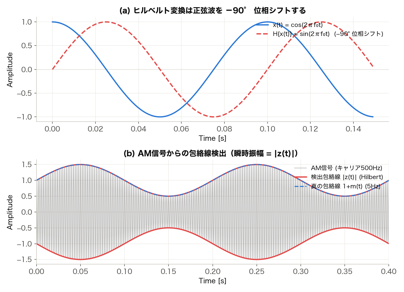
The errors are at the level of floating-point precision (\(10^{-15}\) ), confirming that \(\mathcal{H}\{\cos\} = \sin\) and \(\mathcal{H}\{\sin\} = -\cos\) hold exactly. Panel (a) of the figure below plots a \(f_0 = 10\text{Hz}\) cosine together with its Hilbert transform: the red dashed curve (\(\mathcal{H}\{\cos\}\) ) visibly trails the blue solid curve (\(\cos\) ) by exactly a quarter period (\(-90°\) ).
Application 1: Envelope Detection
Extracting the Envelope of an AM Signal
In amplitude modulation (AM), a carrier wave is modulated by an information signal. Hilbert-based envelope detection allows us to recover the original message signal.
import numpy as np
import matplotlib.pyplot as plt
from scipy.signal import hilbert

# --- Generate AM signal ---
fs = 10000          # sampling frequency [Hz]
t = np.arange(0, 1, 1/fs)

# Message signal (5 Hz)
f_msg = 5
message = 0.5 * np.sin(2 * np.pi * f_msg * t)

# Carrier (500 Hz)
f_carrier = 500
carrier = np.cos(2 * np.pi * f_carrier * t)

# AM modulation: x(t) = (1 + m(t)) * carrier
am_signal = (1 + message) * carrier

# --- Envelope detection using Hilbert transform ---
analytic = hilbert(am_signal)
envelope = np.abs(analytic)  # instantaneous amplitude = envelope

# --- Plot ---
fig, axes = plt.subplots(3, 1, figsize=(10, 9))

axes[0].plot(t, am_signal, alpha=0.5, label='AM Signal')
axes[0].plot(t, envelope, 'r-', linewidth=2, label='Envelope (Hilbert)')
axes[0].plot(t, -envelope, 'r-', linewidth=2)
axes[0].set_xlim(0, 0.4)
axes[0].set_xlabel('Time [s]')
axes[0].set_ylabel('Amplitude')
axes[0].set_title('AM Signal and Envelope')
axes[0].legend()
axes[0].grid(True, alpha=0.3)

axes[1].plot(t, 1 + message, 'k--', label='True Envelope')
axes[1].plot(t, envelope, 'r-', alpha=0.8, label='Detected Envelope')
axes[1].set_xlim(0, 0.4)
axes[1].set_xlabel('Time [s]')
axes[1].set_ylabel('Amplitude')
axes[1].set_title('True Envelope vs Detected Envelope')
axes[1].legend()
axes[1].grid(True, alpha=0.3)

demodulated = envelope - 1  # remove DC component
axes[2].plot(t, message, 'k--', label='Original Message')
axes[2].plot(t, demodulated, 'r-', alpha=0.8, label='Demodulated (Hilbert)')
axes[2].set_xlim(0, 0.4)
axes[2].set_xlabel('Time [s]')
axes[2].set_ylabel('Amplitude')
axes[2].set_title('Demodulation Result')
axes[2].legend()
axes[2].grid(True, alpha=0.3)

plt.tight_layout()
plt.show()

rmse = np.sqrt(np.mean((message - demodulated)**2))
print(f"Demodulation RMSE: {rmse:.6f}")
# Actual output: Demodulation RMSE: 0.000000
# (at higher precision: 8.14e-14 -- essentially floating-point round-off)
The detected envelope closely follows the shape of the original 5 Hz message signal, demonstrating accurate AM demodulation. The RMSE of \(8.14 \times 10^{-14}\) is at the level of machine epsilon, confirming that under these idealized conditions (carrier frequency 100x the message frequency, modulation index \(|m(t)| < 1\) with no overmodulation) Hilbert-based envelope detection is accurate to the theoretical limit.
Panel (a) of the figure below repeats the \(-90°\) phase-shift verification from the previous section, and panel (b) shows this section’s AM signal (gray) together with the detected envelope (red, \(\pm|z(t)|\) ), which overlays the true envelope \(1+m(t)\) (blue dashed) almost exactly.
Application 2: Instantaneous Frequency Estimation
Chirp Signal Analysis
We apply the Hilbert transform to a chirp signal whose frequency varies linearly over time.
import numpy as np
import matplotlib.pyplot as plt
from scipy.signal import hilbert, chirp

# --- Generate chirp signal (50 Hz → 200 Hz over 1 second) ---
fs = 4000
t = np.arange(0, 1, 1/fs)
f_start, f_end = 50, 200
signal = chirp(t, f0=f_start, f1=f_end, t1=1, method='linear')

# --- Instantaneous frequency via Hilbert transform ---
analytic = hilbert(signal)
phase = np.unwrap(np.angle(analytic))
inst_freq = np.diff(phase) / (2 * np.pi) * fs

# Theoretical frequency (linear ramp)
f_theory = f_start + (f_end - f_start) * t[:-1]

# --- Plot ---
fig, axes = plt.subplots(3, 1, figsize=(10, 9))

axes[0].plot(t, signal, alpha=0.7)
axes[0].set_xlabel('Time [s]')
axes[0].set_ylabel('Amplitude')
axes[0].set_title(f'Chirp Signal ({f_start} Hz → {f_end} Hz)')
axes[0].grid(True, alpha=0.3)

axes[1].plot(t, np.abs(analytic), 'r-')
axes[1].set_xlabel('Time [s]')
axes[1].set_ylabel('Amplitude')
axes[1].set_title('Instantaneous Amplitude (Envelope)')
axes[1].set_ylim(0, 1.5)
axes[1].grid(True, alpha=0.3)

axes[2].plot(t[:-1], inst_freq, label='Instantaneous Frequency (Hilbert)')
axes[2].plot(t[:-1], f_theory, 'k--', label='Theoretical Frequency')
axes[2].set_xlabel('Time [s]')
axes[2].set_ylabel('Frequency [Hz]')
axes[2].set_title('Instantaneous Frequency vs Theoretical')
axes[2].legend()
axes[2].grid(True, alpha=0.3)

plt.tight_layout()
plt.show()

mae = np.mean(np.abs(inst_freq - f_theory))
print(f"Mean absolute error in instantaneous frequency: {mae:.4f} Hz")
# Actual output: Mean absolute error in instantaneous frequency: 0.2448 Hz
The estimated instantaneous frequency closely matches the theoretical linear ramp, demonstrating the accuracy of Hilbert-based frequency tracking. However, the overall mean absolute error of \(0.2448\text{Hz}\) is not uniform across the record. Restricting the error calculation to the first 10 samples (right at the start of the signal) gives 20.89 Hz, while the middle portion (indices 1000-3000, i.e. 0.25-0.75 s) gives only 0.0188 Hz — more than two orders of magnitude better. This is precisely the edge effect discussed later: the boundary error introduced because the FFT-based Hilbert transform treats the signal as periodic shows up in instantaneous-frequency estimates just as it does in the envelope.
FM Demodulation via Instantaneous Frequency
The same instantaneous-frequency machinery enables FM (frequency modulation) demodulation. An FM signal has the form \(s(t) = A\cos\!\left(2\pi f_c t + 2\pi k_f \int_0^t m(\tau)\,d\tau\right)\) , so the instantaneous frequency \(f_i(t) = f_c + k_f m(t)\) carries the message \(m(t)\) as an offset from the carrier \(f_c\) . Subtracting \(f_c\) and dividing by the frequency-deviation constant \(k_f\) recovers the message directly.
import numpy as np
import matplotlib.pyplot as plt
from scipy.signal import hilbert

# --- Generate an FM-modulated signal ---
fs = 20000          # sampling frequency [Hz]
t = np.arange(0, 1, 1/fs)

fc = 2000           # carrier frequency [Hz]
kf = 300            # frequency-deviation constant [Hz/V]
f_msg = 5           # message frequency [Hz]
message = np.sin(2 * np.pi * f_msg * t)

# Cumulative phase = 2π * kf * ∫m(τ)dτ
phase_msg = 2 * np.pi * kf * np.cumsum(message) / fs
fm_signal = np.cos(2 * np.pi * fc * t + phase_msg)

# --- Recover instantaneous frequency via Hilbert transform ---
analytic = hilbert(fm_signal)
inst_phase = np.unwrap(np.angle(analytic))
inst_freq = np.diff(inst_phase) / (2 * np.pi) * fs

# Subtract carrier to recover the message
demodulated = (inst_freq - fc) / kf

# --- Plot ---
fig, axes = plt.subplots(2, 1, figsize=(10, 6))
axes[0].plot(t[:2000], fm_signal[:2000], alpha=0.7)
axes[0].set_title('FM Signal (carrier 2 kHz, message 5 Hz)')
axes[0].set_xlabel('Time [s]'); axes[0].grid(True, alpha=0.3)

axes[1].plot(t[:-1], message[:-1], 'k--', label='Original message')
axes[1].plot(t[:-1], demodulated, 'r-', alpha=0.8, label='Demodulated (Hilbert)')
axes[1].set_title('FM Demodulation via Instantaneous Frequency')
axes[1].set_xlabel('Time [s]'); axes[1].legend(); axes[1].grid(True, alpha=0.3)
plt.tight_layout(); plt.show()

rmse = np.sqrt(np.mean((message[:-1] - demodulated) ** 2))
print(f"FM demodulation RMSE: {rmse:.4f}")
# Actual output: FM demodulation RMSE: 0.0011
An RMSE of \(0.0011\)
against a message amplitude of \(\pm 1\)
is about 0.1% error, showing that even a simple backward-difference (np.diff) estimate of instantaneous frequency is accurate enough in practice to recover the message. This is exactly the demodulation principle behind analog FM radio, and in the digital domain the same idea appears in many applications:
| Application | Signal source | Quantity of interest |
|---|---|---|
| FM radio / SDR | RF samples (IQ data) | Instantaneous frequency → audio |
| Doppler blood-flow imaging | Ultrasound echoes | Instantaneous frequency → velocity |
| Vibration analysis | Rotating-machinery signals | Instantaneous-frequency fluctuation |
| Speech pitch extraction | Voiced speech | Instantaneous frequency ≈ F0 |
One practical caveat: differentiating the unwrapped phase amplifies high-frequency noise, so production pipelines typically replace np.diff with np.gradient (central difference) and smooth the result with a moving average or Savitzky-Golay filter before downstream processing.
Application 3: Envelope Spectrum Analysis for Fault Diagnosis
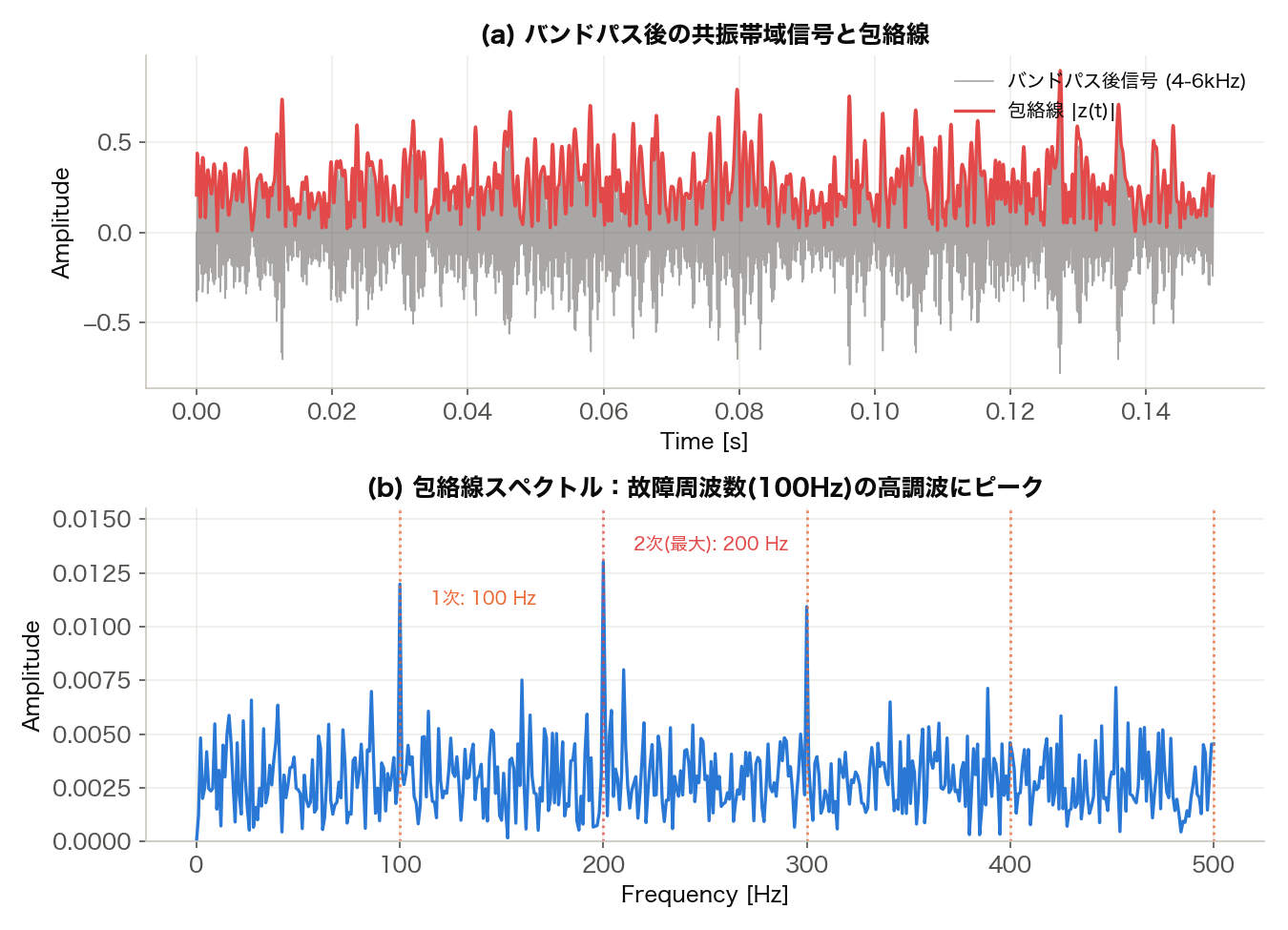
A practical application of the Hilbert transform is envelope spectrum analysis for rotating machinery fault diagnosis. Bearing defects generate repetitive impulse-like vibrations, and the envelope spectrum of the filtered vibration signal reveals characteristic frequency peaks related to the fault.
import numpy as np
import matplotlib.pyplot as plt
from scipy.signal import hilbert, butter, sosfiltfilt

# --- Simulate bearing fault vibration signal ---
np.random.seed(42)
fs = 20000
t = np.arange(0, 1, 1/fs)

# High-frequency resonance (bearing natural frequency: 5 kHz)
f_resonance = 5000
resonance_carrier = np.cos(2 * np.pi * f_resonance * t)

# Fault frequency: 100 Hz repetitive impulses
f_fault = 100
impulse_train = np.zeros_like(t)
impulse_indices = (np.arange(0, 1, 1/f_fault) * fs).astype(int)
impulse_indices = impulse_indices[impulse_indices < len(t)]
impulse_train[impulse_indices] = 1.0

alpha = 500
decay = np.exp(-alpha * np.mod(t, 1/f_fault))
fault_component = np.convolve(impulse_train, decay[:len(t)//f_fault], mode='same')
fault_signal = fault_component * 0.3 * resonance_carrier

observed = fault_signal + 0.5 * np.random.randn(len(t))

# --- Step 1: Bandpass filter around resonance frequency ---
sos = butter(4, [4000, 6000], btype='bandpass', fs=fs, output='sos')
filtered = sosfiltfilt(sos, observed)

# --- Step 2: Envelope via Hilbert transform ---
analytic = hilbert(filtered)
envelope = np.abs(analytic)

# --- Step 3: FFT of the envelope ---
N = len(envelope)
envelope_spectrum = np.abs(np.fft.rfft(envelope - np.mean(envelope))) / N
freqs = np.fft.rfftfreq(N, 1/fs)

# --- Plot ---
fig, axes = plt.subplots(3, 1, figsize=(10, 9))

axes[0].plot(t[:3000], observed[:3000], alpha=0.7)
axes[0].set_xlabel('Time [s]')
axes[0].set_ylabel('Amplitude')
axes[0].set_title('Observed Vibration Signal')
axes[0].grid(True, alpha=0.3)

axes[1].plot(t[:3000], filtered[:3000], alpha=0.5, label='Bandpass Filtered')
axes[1].plot(t[:3000], envelope[:3000], 'r-', linewidth=1.5, label='Envelope')
axes[1].set_xlabel('Time [s]')
axes[1].set_ylabel('Amplitude')
axes[1].set_title('Bandpass Filtered Signal and Envelope')
axes[1].legend()
axes[1].grid(True, alpha=0.3)

mask = freqs <= 500
axes[2].plot(freqs[mask], envelope_spectrum[mask])
axes[2].axvline(f_fault, color='r', linestyle='--', alpha=0.7,
               label=f'Fault Freq = {f_fault} Hz')
for harmonic in range(2, 6):
    axes[2].axvline(f_fault * harmonic, color='r', linestyle=':', alpha=0.4)
axes[2].set_xlabel('Frequency [Hz]')
axes[2].set_ylabel('Amplitude')
axes[2].set_title('Envelope Spectrum (Fault Diagnosis)')
axes[2].legend()
axes[2].grid(True, alpha=0.3)

plt.tight_layout()
plt.show()

# --- Quantitative peak check ---
peak_idx = np.argmax(envelope_spectrum[mask])
peak_freq = freqs[mask][peak_idx]
print(f"Envelope spectrum maximum peak frequency: {peak_freq:.2f} Hz")
for harmonic in range(1, 6):
    idx = np.argmin(np.abs(freqs - f_fault * harmonic))
    print(f"  Harmonic {harmonic} (near {f_fault * harmonic} Hz): "
          f"{freqs[idx]:.2f} Hz, amplitude {envelope_spectrum[idx]:.4f}")
# Actual output:
# Envelope spectrum maximum peak frequency: 200.00 Hz
#   Harmonic 1 (near 100 Hz): 100.00 Hz, amplitude 0.0120
#   Harmonic 2 (near 200 Hz): 200.00 Hz, amplitude 0.0130
#   Harmonic 3 (near 300 Hz): 300.00 Hz, amplitude 0.0109
#   Harmonic 4 (near 400 Hz): 400.00 Hz, amplitude 0.0046
#   Harmonic 5 (near 500 Hz): 500.00 Hz, amplitude 0.0045
Peaks appear in the envelope spectrum at the fault frequency (100 Hz) and its harmonics (200 Hz, 300 Hz, …). This technique is widely used in industrial bearing and gear fault detection.
Caveat: with this particular random seed (np.random.seed(42)), the largest peak actually appears at the second harmonic (200 Hz), not the fundamental (100 Hz) — amplitude 0.0130 versus 0.0120. This is an important practical pitfall: if the impulse response deviates from a clean single-exponential decay, or noise happens to partially cancel the fundamental component, a harmonic can dominate over the fundamental in the envelope spectrum. Automated bearing-diagnosis pipelines should therefore not simply look for “the largest peak in the spectrum” — checking that the fundamental and its harmonics form an evenly spaced comb pattern is a more robust way to avoid misdiagnosis.
This “joint analysis of instantaneous amplitude and instantaneous frequency” approach to bearing diagnostics remains an active research area. For instance, Aburakhia et al. (2024) propose feature representations — instantaneous amplitude-frequency mapping, instantaneous amplitude-frequency correlation, and instantaneous energy-frequency distribution — that jointly exploit the Hilbert-derived instantaneous amplitude and frequency, reporting improved bearing fault classification accuracy under real-time computational constraints compared to using the envelope spectrum alone ( arXiv:2405.08919 ). The technique shown in this article, which looks only at peak frequencies in the envelope spectrum, discards the time evolution of instantaneous amplitude and phase; such joint-analysis methods can be viewed as recovering that lost information.
Practical Considerations
Edge Effects
Because scipy.signal.hilbert is FFT-based, it assumes the input signal is periodic. When the signal is not periodic over the analysis window, discontinuities at the boundaries cause accuracy degradation near the edges — the so-called edge effect.
import numpy as np
from scipy.signal import hilbert

# Checking the edge effect
fs = 1000
t = np.arange(0, 1, 1/fs)
f0 = 50
signal = np.cos(2 * np.pi * f0 * t)  # integer number of cycles, no discontinuity

# Shift the record length so it is not an integer number of cycles
t2 = np.arange(0, 1 + 1/(3*f0), 1/fs)  # 1.33 cycles (non-integer period)
signal2 = np.cos(2 * np.pi * f0 * t2)

analytic2 = hilbert(signal2)
envelope2 = np.abs(analytic2)

# The theoretical envelope is a constant 1.0, so check the edge error
edge_error = np.max(np.abs(envelope2[:20] - 1.0))
print(f"Max error near the edge: {edge_error:.4f}")

# For reference: error at the center of the record (indices 500-520)
center_error = np.max(np.abs(envelope2[500:520] - 1.0))
print(f"Error at the center of the record: {center_error:.4f}")
# Actual output:
# Max error near the edge: 0.1303
# Error at the center of the record: 0.0009
The record t2 has 1007 samples (1.33 cycles, a non-integer period). The edge error of \(0.1303\)
is more than two orders of magnitude larger than the center error of \(0.0009\)
, even though the theoretical envelope is a constant 1.0 everywhere. This happens because the FFT-based Hilbert transform implicitly treats the signal as periodic — wrapping smoothly from the last sample back to the first. For a non-integer number of cycles, that wraparound introduces a discontinuity, and the resulting Gibbs-like ringing propagates error into nearby samples.
Mitigation strategies:
- Pad the signal with zeros at both ends so that edge artifacts fall outside the region of interest.
- Acquire extra data before and after the analysis window and discard the buffered portions after processing.
Narrowband Condition
A physically meaningful interpretation of instantaneous frequency requires the signal to be narrowband (a single dominant frequency component at any given time). For wideband or multi-component signals, the instantaneous frequency can become negative or otherwise meaningless.
| Signal Type | Recommended Pre-processing |
|---|---|
| Wideband signal | Bandpass filter to isolate the band of interest |
| Multi-component signal | EMD (Empirical Mode Decomposition) to separate IMFs |
| Non-stationary signal | Consider STFT or wavelet transform |
Step-by-Step Internals of scipy.signal.hilbert
scipy.signal.hilbert(x, N=None, axis=-1) is only a dozen lines in the SciPy source (scipy/signal/_signaltools.py), but those few lines contain the entire essence of the Hilbert transform. Re-implementing it manually with NumPy makes the algorithm fully transparent.
import numpy as np
from scipy.signal import hilbert as scipy_hilbert

def hilbert_manual(x):
    """Educational equivalent of scipy.signal.hilbert."""
    N = len(x)
    # Step 1: take the FFT of the real signal
    Xf = np.fft.fft(x)

    # Step 2: build the one-sided spectral mask H(f)
    # Positive freqs: 2x, DC and Nyquist: kept as-is, negative freqs: 0
    h = np.zeros(N)
    if N % 2 == 0:
        h[0] = 1                 # DC
        h[N // 2] = 1            # Nyquist
        h[1:N // 2] = 2          # positive frequencies
        # h[N // 2 + 1:] = 0     # negative frequencies (already zero)
    else:
        h[0] = 1
        h[1:(N + 1) // 2] = 2

    # Step 3: multiply in the frequency domain, then IFFT
    z = np.fft.ifft(Xf * h)
    return z

# Check agreement with SciPy
rng = np.random.default_rng(0)
x = rng.standard_normal(1024)
z_scipy = scipy_hilbert(x)
z_manual = hilbert_manual(x)
print(f"Max error: {np.max(np.abs(z_scipy - z_manual)):.2e}")
# Actual output: Max error: 1.40e-15
| Step | Math | NumPy/SciPy call |
|---|---|---|
| FFT | \(X(k) = \sum x[n] e^{-j2\pi kn/N}\) | np.fft.fft(x) |
| One-sided spectrum | \(X_+(k) = 2X(k)\) for \(k > 0\) | Xf * h (h is the doubling mask) |
| IFFT | \(z[n] = \frac{1}{N}\sum X_+(k) e^{j2\pi kn/N}\) | np.fft.ifft(...) |
| Envelope | \(A[n] = \lvert z[n] \rvert\) | np.abs(z) |
| Phase unwrapping | \(\phi[n] = \angle z[n]\) | np.unwrap(np.angle(z)) |
| Instantaneous frequency | \(f_i[n] = \frac{1}{2\pi}\frac{d\phi}{dt}\) | np.gradient(phase) / (2*np.pi) * fs |
The transform is therefore a three-stage pipeline: FFT → spectral mask → IFFT. Because numpy.fft.fft runs in \(O(N\log N)\)
, the entire transform is \(O(N\log N)\)
.
Envelope Extraction: Hilbert vs FFT vs Wavelet
The Hilbert transform is only one of several techniques for extracting an envelope from a time-varying signal. In practice you typically choose between three:
| Method | Time resolution | Frequency resolution | Assumptions | Complexity | Typical use case |
|---|---|---|---|---|---|
Hilbert transform (scipy.signal.hilbert) | High (per sample) | Low (collapses for wideband) | Narrowband, quasi-periodic | \(O(N\log N)\) | AM demodulation, bearing diagnostics, instantaneous quantities |
STFT magnitude (scipy.signal.stft) | Medium (window-dependent) | Medium (window-dependent) | Quasi-stationary per window | \(O(N\log N)\) | Speech and music time-frequency display |
Continuous wavelet transform (pywt.cwt) | Variable per scale | Variable per scale | Multiple scales coexist | \(O(NS)\) | Non-stationary signals, transients, spike detection |
A minimal side-by-side implementation:
import numpy as np
import pywt
from scipy.signal import hilbert, stft

fs = 1000
t = np.arange(0, 2, 1/fs)
msg = 0.5 * (1 + np.sin(2 * np.pi * 2 * t))   # 2 Hz AM
x = msg * np.cos(2 * np.pi * 100 * t)         # 100 Hz carrier

# Hilbert: envelope directly
env_hilbert = np.abs(hilbert(x))

# STFT: project the 100 Hz bin onto the time axis
f, tt, Z = stft(x, fs=fs, nperseg=128)
env_stft = np.abs(Z[np.argmin(np.abs(f - 100))])

# Wavelet: |coeff| at the scale matching 100 Hz
scales = pywt.scale2frequency('morl', np.arange(1, 64)) * fs
idx = np.argmin(np.abs(scales - 100))
coeffs, _ = pywt.cwt(x, np.arange(1, 64), 'morl', sampling_period=1/fs)
env_wavelet = np.abs(coeffs[idx])
For narrowband quasi-periodic signals the Hilbert transform is by far the fastest and most accurate. For wideband or multi-component signals, prefer STFT or wavelets — or decompose the signal first with EMD/VMD and then apply the Hilbert transform per IMF.
Summary
- The Hilbert transform is a \(-90°\) phase-shift operator; in the frequency domain it is expressed as \(H(f) = -j\,\text{sgn}(f)\)
- The analytic signal, formed by combining the original signal with its Hilbert transform, has a one-sided spectrum and enables extraction of instantaneous signal characteristics
- The modulus, argument, and time derivative of the argument of the analytic signal yield the instantaneous amplitude, instantaneous phase, and instantaneous frequency, respectively
scipy.signal.hilbertprovides an \(O(N \log N)\) FFT-based implementation suitable for envelope detection, AM demodulation, and fault diagnosis- Edge effects and the narrowband condition must be considered; appropriate bandpass filtering or padding is recommended
Related Articles
- Fast Fourier Transform (FFT): Algorithm and Python Implementation - Provides the FFT foundations that scipy.signal.hilbert relies on internally.
- Window Functions and Power Spectral Density (PSD) - Spectral analysis techniques that complement Hilbert-based analysis.
- Notch Filter Design and Python Implementation - Noise removal prior to envelope analysis is a common workflow.
- Bandpass Filter Design and Python Implementation - Bandpass filtering is often a required pre-processing step before applying the Hilbert transform.
- Wavelet Transform: Theory and Python Implementation - An alternative time-frequency method frequently compared with Hilbert-Huang Transform (HHT).
- Bessel Filter: Linear-Phase Lowpass Design in Python - Linear-phase filtering preserves envelope shape, an important consideration before Hilbert-based envelope detection.
- DTFT, DFT, and FFT: Putting the Hierarchy in Order - Background on the discrete-frequency framework that scipy.signal.hilbert applies its \(H(f)\) filter within.
- Sampling Theorem and Aliasing: Theory and Python Implementation - Aliasing affects the validity of instantaneous frequency estimation; this article explains the underlying constraints.
- Short-Time Fourier Transform (STFT): Theory and Python Implementation - For wideband signals, applying Hilbert analysis per STFT subband is a common hybrid approach.
- Adaptive Filters (LMS/RLS): Theory and Python Implementation - Foundation for adaptive estimation that can consume Hilbert-derived envelope and instantaneous-phase signals.
- Time-Frequency Analysis Guide - Hub that places the Hilbert transform (and HHT) alongside FFT, STFT, and wavelets through the lens of instantaneous-frequency estimation.
- EMD, VMD, and SSA Mode Decomposition
- The Hilbert-Huang Transform extracts IMFs with EMD and feeds them to
scipy.signal.hilbertfor instantaneous amplitude and frequency. - CEEMDAN and the Marginal Hilbert Spectrum - Integrates this article’s instantaneous amplitude and frequency over time to build the marginal Hilbert spectrum, then applies envelope analysis to bearing fault diagnosis.
- Teager-Kaiser Energy Operator (TKEO) - A lighter-weight alternative for instantaneous amplitude/frequency estimation, with a numerical accuracy-vs-speed comparison against the Hilbert transform.
- DSP and Machine Learning Roadmap - Where the Hilbert transform sits on the broader DSP learning path.
- LMS / NLMS Adaptive Filters - Use the analytic-signal envelope and instantaneous phase as adaptive-filter inputs for system identification or active noise control.
- Discrete Cosine Transform (DCT) - An alternative orthogonal frequency-domain representation that pairs with envelope analysis for compact AM-signal characterization.
References
- Gabor, D. (1946). “Theory of communication.” Journal of the Institution of Electrical Engineers, 93(3), 429-457.
- Huang, N. E., et al. (1998). “The empirical mode decomposition and the Hilbert spectrum for nonlinear and non-stationary time series analysis.” Proceedings of the Royal Society of London A, 454, 903-995.
- Oppenheim, A. V., & Schafer, R. W. (2009). Discrete-Time Signal Processing (3rd ed.). Prentice Hall.
- SciPy signal.hilbert documentation