Introduction
A fundamental challenge in speech signal analysis is separating the vibration of the vocal folds (source) from the shape of the vocal tract (filter). Under the source-filter model, a speech signal is represented as the convolution of a glottal pulse train with the vocal-tract transfer function. In the frequency domain this convolution becomes a product, and taking the logarithm converts the product to a sum — and that is the central idea of cepstrum analysis.
The cepstrum is a portmanteau coined in 1963 by Bogert, Healy, and Tukey as an anagram of “spectrum.” All cepstrum-specific terminology (quefrency, liftering, etc.) is likewise derived from anagrams of spectral terms, reflecting the unique concept of a “spectrum of a spectrum.”
This article systematically covers the mathematical definition of the cepstrum, spectral envelope estimation, pitch estimation, and applications to MFCC (Mel-Frequency Cepstral Coefficients), with Python implementations throughout.
Source-Filter Model
Mathematical Model of Speech Production
A speech signal \(s[n]\) is described by the following source-filter model:
\[s[n] = e[n] * h[n] \tag{1}\]where:
- \(e[n]\) : source signal (glottal pulse train or fricative noise)
- \(h[n]\) : vocal-tract impulse response (vocal-tract filter)
- \(*\) : convolution operator
Frequency-Domain Representation
Convolution in the time domain corresponds to multiplication in the frequency domain via the Fourier transform:
\[S(f) = E(f) \cdot H(f) \tag{2}\]Taking the logarithm converts multiplication into addition:
\[\log |S(f)| = \log |E(f)| + \log |H(f)| \tag{3}\]where:
- \(\log |S(f)|\) : observed log-amplitude spectrum
- \(\log |E(f)|\) : log spectrum of the source (rapidly varying component: harmonics)
- \(\log |H(f)|\) : log spectral envelope of the vocal tract (slowly varying component)
Applying the inverse Fourier transform to this additive relation defines the cepstrum.
Definition of the Cepstrum
Real Cepstrum
The real cepstrum of a signal \(x[n]\) is defined as:
\[c[q] = \mathcal{F}^{-1}\{\log |\mathcal{F}\{x[n]\}|\} \tag{4}\] \[= \mathcal{F}^{-1}\{\log |X(f)|\} \tag{5}\]The parameter \(q\) is called the quefrency, the analogue of “frequency” in the spectral domain (units: seconds).
The computation proceeds as follows:
- Compute the DFT of \(x[n]\) : \(X[k] = \text{DFT}\{x[n]\}\)
- Compute the amplitude spectrum: \(|X[k]|\)
- Take the logarithm: \(\log |X[k]|\)
- Compute the inverse DFT: \(c[q] = \text{IDFT}\{\log |X[k]|\}\)
Complex Cepstrum
The more general complex cepstrum retains phase information:
\[\hat{c}[q] = \mathcal{F}^{-1}\{\log X(f)\} = \mathcal{F}^{-1}\{\log |X(f)| + j \angle X(f)\} \tag{6}\]The complex cepstrum requires phase unwrapping and is computationally more involved, but it enables perfect reconstruction (recovery of the original signal).
Physical Interpretation of Quefrency
Quefrency \(q\) [s] corresponds to the “period” of the log spectrum:
- Low-quefrency components (small \(q\) ): slowly varying features of the log spectrum → vocal-tract spectral envelope \(\log |H(f)|\)
- High-quefrency components (\(q = 1/f_0\) ): fine-grained harmonic structure from the source → peak corresponding to fundamental frequency \(f_0\)
By selecting an appropriate quefrency range, one can separate the source from the vocal-tract characteristics.
Liftering
Windowing in the cepstral domain is called liftering (an anagram of “filtering”):
\[\tilde{c}[q] = c[q] \cdot l[q] \tag{7}\]where \(l[q]\) is a window function called a lifter:
- Low-pass lifter (passing only low quefrencies): extracts the vocal-tract spectral envelope
- High-pass lifter (passing only high quefrencies): extracts the source components (harmonics)
Applying a low-pass lifter and then taking the inverse transform yields the log spectral envelope; applying a high-pass lifter yields the log spectrum of the source.
Python Implementation
Basic Cepstrum Computation
import numpy as np
import matplotlib.pyplot as plt
from scipy.signal import lfilter

def compute_real_cepstrum(signal, n_fft=None):
    """
    Compute the real cepstrum.

    Parameters
    ----------
    signal : np.ndarray
        Input signal
    n_fft : int, optional
        FFT size (defaults to the next power of two above the signal length)

    Returns
    -------
    cepstrum : np.ndarray
        Real cepstrum
    """
    if n_fft is None:
        n_fft = 2 ** int(np.ceil(np.log2(len(signal))))
    # Step 1: DFT
    X = np.fft.fft(signal, n=n_fft)
    # Step 2: log of the amplitude spectrum
    log_spec = np.log(np.abs(X) + 1e-10)
    # Step 3: inverse DFT (take real part only)
    cepstrum = np.fft.ifft(log_spec).real
    return cepstrum


def formant_ar_coeffs(formants_bw, fs):
    """
    Design a stable AR filter from formant frequencies and bandwidths.

    Each formant (F, BW) is modeled as a second-order resonator (a complex
    conjugate pole pair), with the pole radius r = exp(-pi*BW/fs) kept
    strictly below 1 so that lfilter never diverges. Handing lfilter
    hand-picked AR coefficients can easily produce an unstable filter —
    this pitfall is examined quantitatively in "Implementation Edge Cases
    and Caveats" below.
    """
    poly = np.array([1.0])
    for F, BW in formants_bw:
        r = np.exp(-np.pi * BW / fs)
        theta = 2 * np.pi * F / fs
        second_order = np.array([1.0, -2 * r * np.cos(theta), r**2])
        poly = np.convolve(poly, second_order)
    return poly


# --- Synthesize a voiced speech signal ---
fs = 8000
T = 0.05      # 50 ms frame
t = np.arange(0, T, 1/fs)
f0 = 150      # fundamental frequency [Hz]

# Glottal pulse train (approximation of a glottal pulse)
glottal = np.zeros_like(t)
period_samples = int(fs / f0)
for i in range(0, len(t), period_samples):
    if i + 30 < len(t):
        glottal[i:i+30] = np.exp(-np.arange(30) * 0.15)

# Vocal-tract filter: AR(4) model with formants F1=800 Hz (bandwidth 80 Hz)
# and F2=1200 Hz (bandwidth 100 Hz)
ar_coeffs = formant_ar_coeffs([(800, 80), (1200, 100)], fs)
print("AR coefficients:", np.round(ar_coeffs, 4))
print("Pole magnitudes (all < 1 means stable):", np.round(np.abs(np.roots(ar_coeffs)), 4))

voiced = lfilter([1.0], ar_coeffs, glottal)
voiced = voiced / np.max(np.abs(voiced) + 1e-8)

# --- Cepstrum computation ---
n_fft = 512
cepstrum = compute_real_cepstrum(voiced, n_fft=n_fft)
quefrency = np.arange(n_fft) / fs * 1000   # in ms

# Log spectrum
X = np.fft.fft(voiced, n=n_fft)
log_spec = np.log(np.abs(X[:n_fft//2 + 1]) + 1e-10)
freqs = np.fft.rfftfreq(n_fft, 1/fs)

# Top 5 cepstrum peaks in the 1-20 ms quefrency range
idx_range = np.where((quefrency[:n_fft//2] > 1) & (quefrency[:n_fft//2] < 20))[0]
top5 = idx_range[np.argsort(cepstrum[idx_range])[::-1][:5]]
for idx in top5:
    print(f"q={quefrency[idx]:.3f} ms, cepstrum={cepstrum[idx]:.5f}")

# --- Plot ---
fig, axes = plt.subplots(3, 1, figsize=(12, 10))

# Time waveform
axes[0].plot(t * 1000, voiced)
axes[0].set_xlabel('Time [ms]')
axes[0].set_ylabel('Amplitude')
axes[0].set_title(f'Synthetic Voice: F0={f0} Hz, Formants F1≈800Hz, F2≈1200Hz')
axes[0].grid(True, alpha=0.3)

# Log amplitude spectrum
axes[1].plot(freqs, log_spec)
axes[1].set_xlabel('Frequency [Hz]')
axes[1].set_ylabel('Log Magnitude')
axes[1].set_title('Log Amplitude Spectrum')
axes[1].set_xlim(0, 4000)
axes[1].grid(True, alpha=0.3)

# Cepstrum
axes[2].plot(quefrency[:n_fft//2], cepstrum[:n_fft//2])
axes[2].axvline(x=1000/f0, color='r', linestyle='--',
                label=f'1/F0 = {1000/f0:.1f} ms')
axes[2].set_xlabel('Quefrency [ms]')
axes[2].set_ylabel('Cepstral Amplitude')
axes[2].set_title('Real Cepstrum: Pitch peak visible at 1/F0')
axes[2].set_xlim(0, 20)
axes[2].legend()
axes[2].grid(True, alpha=0.3)

plt.tight_layout()
plt.show()
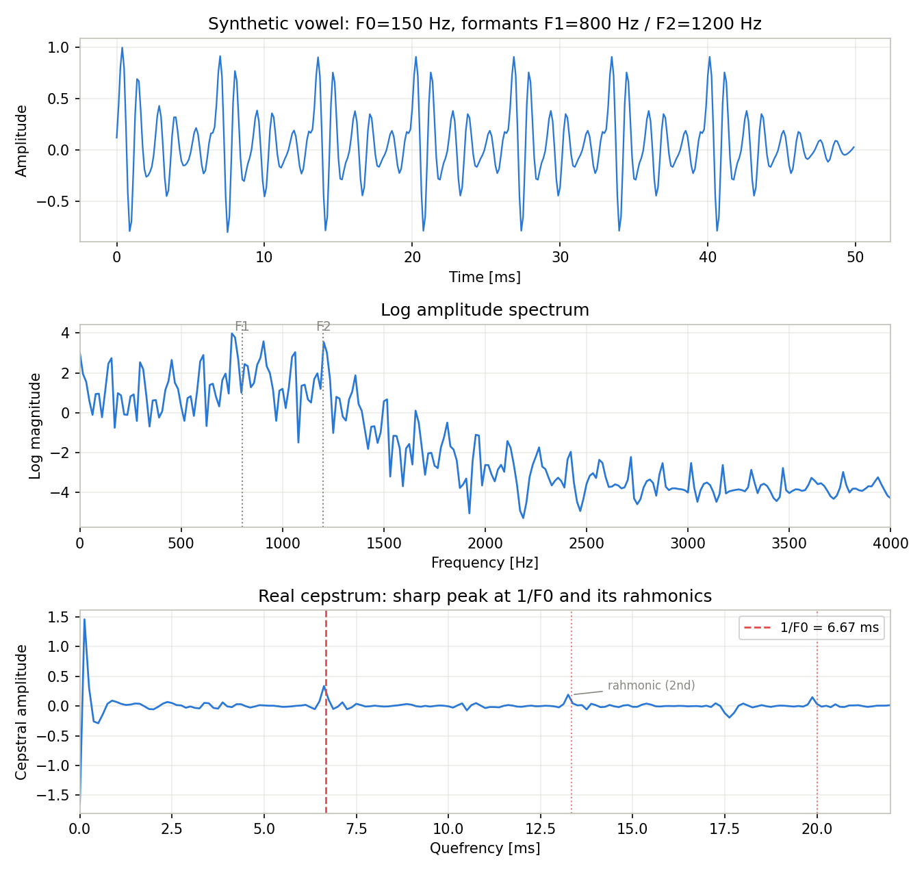
Running this code confirms that the AR coefficients are [1.0, -2.6983, 3.6359, -2.5110, 0.8682] and the pole magnitudes are [0.9615, 0.9615, 0.9691, 0.9691] — all below 1 (inside the unit circle), so the filter is stable. Searching for the top cepstrum peaks in the 1-20 ms quefrency range yields:
| Quefrency [ms] | Cepstral amplitude | Corresponding component |
|---|---|---|
| 6.625 | 0.3377 | Fundamental-frequency peak (nearest bin to the theoretical \(1/f_0=6.667\) ms) |
| 13.250 | 0.1918 | 2nd rahmonic (\(2/f_0\) ) |
| 19.875 | 0.1489 | 3rd rahmonic (\(3/f_0\) ) |
| 6.750 | 0.1090 | Bin adjacent to the main peak |
| 6.500 | 0.0770 | Bin adjacent to the main peak |
The largest peak falls in the bin closest to the theoretical value (6.625 ms, given the quefrency resolution \(1/f_s = 0.125\) ms), and decaying peaks also appear at integer multiples (13.25 ms, 19.875 ms). Because the source is a periodic pulse train, the log spectrum oscillates at intervals of the fundamental frequency, and its Fourier transform — the cepstrum — produces a secondary peak, called a rahmonic, at every integer multiple of \(1/f_0\) .
Spectral Envelope Extraction via Liftering
import numpy as np
import matplotlib.pyplot as plt
from scipy.signal import lfilter

def lifter_cepstrum(cepstrum, cutoff_ms, fs, n_fft):
    """
    Extract the spectral envelope using a low-pass lifter.

    Parameters
    ----------
    cepstrum : np.ndarray
        Input cepstrum (length n_fft)
    cutoff_ms : float
        Low-pass lifter cutoff [ms]
    fs : float
        Sampling frequency
    n_fft : int
        FFT size

    Returns
    -------
    envelope_log : np.ndarray
        Log spectral envelope (length n_fft//2 + 1)
    """
    cutoff_samples = int(cutoff_ms * fs / 1000)

    # Low-pass lifter
    lifter = np.zeros(n_fft)
    lifter[:cutoff_samples] = 1.0
    lifter[-cutoff_samples+1:] = 1.0  # symmetric component

    # Liftering
    liftered = cepstrum * lifter

    # Inverse DFT → log spectral envelope
    envelope_log = np.fft.fft(liftered, n=n_fft).real
    return envelope_log[:n_fft//2 + 1]


# --- Run after the code above ---
cutoff_list = [2.0, 3.5, 5.0]   # cutoff values in ms

fig, axes = plt.subplots(len(cutoff_list), 1, figsize=(12, 10))

for ax, cutoff_ms in zip(axes, cutoff_list):
    envelope = lifter_cepstrum(cepstrum, cutoff_ms, fs, n_fft)

    ax.plot(freqs, log_spec, alpha=0.5, label='Log spectrum', color='steelblue')
    ax.plot(freqs, envelope, linewidth=2, label=f'Envelope (cutoff={cutoff_ms} ms)',
            color='red')
    ax.set_xlabel('Frequency [Hz]')
    ax.set_ylabel('Log Magnitude')
    ax.set_title(f'Spectral Envelope Extraction via Low-pass Liftering ({cutoff_ms} ms)')
    ax.set_xlim(0, 4000)
    ax.legend()
    ax.grid(True, alpha=0.3)

plt.tight_layout()
plt.show()
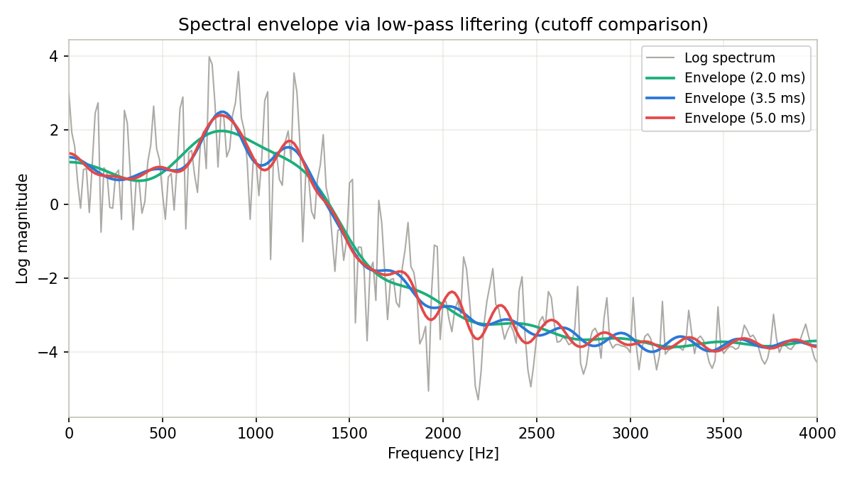
Running the code above and comparing the RMSE (root-mean-square error) between each envelope and the original log spectrum, along with the formant peaks detected from the envelope (in the 100-3000 Hz range, via scipy.signal.argrelextrema), gives:
| Cutoff [ms] | RMSE | Detected peaks [Hz] |
|---|---|---|
| 2.0 | 0.877 | 812.5 (F1 only — F2 is smoothed away and not detected) |
| 3.5 | 0.854 | 812.5, 1171.9 (both F1 and F2 detected) |
| 5.0 | 0.840 | 812.5, 1171.9 (both detected; slightly more high-frequency ripple) |
At a 2.0 ms cutoff, too much low-quefrency content is removed, so the two resonances F1 (≈800 Hz) and F2 (≈1200 Hz) merge into a single smooth bump and F2’s information is lost. At 3.5 ms and 5.0 ms both formants are correctly separated, but pushing the cutoff out to 5.0 ms approaches the quefrency of the source periodicity (\(1/f_0 \approx 6.67\) ms), producing slightly more high-frequency ripple (residual harmonics). This confirms quantitatively that the common rule of thumb — a 3-4 ms cutoff — holds for this vowel sample as well.
Pitch Estimation via Cepstrum
import numpy as np
import matplotlib.pyplot as plt
from scipy.signal import lfilter

def formant_ar_coeffs(formants_bw, fs):
    """Design a stable AR filter from formant frequencies and bandwidths (helper defined earlier)."""
    poly = np.array([1.0])
    for F, BW in formants_bw:
        r = np.exp(-np.pi * BW / fs)
        theta = 2 * np.pi * F / fs
        second_order = np.array([1.0, -2 * r * np.cos(theta), r**2])
        poly = np.convolve(poly, second_order)
    return poly


def cepstrum_pitch_detection(signal, fs, fmin=60, fmax=600):
    """
    Detect the fundamental frequency (F0) using the cepstrum.

    Parameters
    ----------
    signal : np.ndarray
        Input speech frame
    fs : float
        Sampling frequency [Hz]
    fmin, fmax : float
        Search range for F0 [Hz]

    Returns
    -------
    f0 : float or None
        Estimated F0 [Hz]
    cepstrum : np.ndarray
        Cepstrum
    quefrency_ms : np.ndarray
        Quefrency axis [ms]
    """
    n_fft = 2 ** int(np.ceil(np.log2(len(signal))))

    # Cepstrum computation
    X = np.fft.fft(signal * np.hanning(len(signal)), n=n_fft)
    log_spec = np.log(np.abs(X) + 1e-10)
    cepstrum = np.fft.ifft(log_spec).real

    # Convert F0 search range to quefrency indices
    q_min = int(fs / fmax)
    q_max = int(fs / fmin)
    q_max = min(q_max, n_fft // 2)

    # Peak detection
    pitch_region = cepstrum[q_min:q_max]
    peak_idx = np.argmax(pitch_region) + q_min
    f0 = fs / peak_idx

    quefrency_ms = np.arange(n_fft) / fs * 1000

    return f0, cepstrum, quefrency_ms


# --- Test estimation at different F0 values ---
fs = 16000
T = 0.04  # 40 ms frame
t = np.arange(0, T, 1/fs)

test_f0s = [120, 180, 250]  # Hz

# Vocal-tract filter: stable AR(4) model with formants F1=700 Hz (bandwidth 80 Hz)
# and F2=1300 Hz (bandwidth 120 Hz)
ar = formant_ar_coeffs([(700, 80), (1300, 120)], fs)

fig, axes = plt.subplots(len(test_f0s), 2, figsize=(14, 10))

for i, f0_true in enumerate(test_f0s):
    np.random.seed(i)
    # Synthesize voiced speech
    period = int(fs / f0_true)
    glottal = np.zeros_like(t)
    for k in range(0, len(t), period):
        if k + 20 < len(t):
            glottal[k:k+20] = np.exp(-np.arange(20) * 0.2)

    voice = lfilter([1.0], ar, glottal)
    voice = voice / (np.max(np.abs(voice)) + 1e-8)
    voice += 0.02 * np.random.randn(len(t))

    f0_est, cep, q_ms = cepstrum_pitch_detection(voice, fs)
    n_fft = len(cep)
    err_pct = abs(f0_est - f0_true) / f0_true * 100
    print(f"True F0={f0_true} Hz -> Estimated F0={f0_est:.2f} Hz (error {err_pct:.2f}%)")

    axes[i, 0].plot(t * 1000, voice)
    axes[i, 0].set_xlabel('Time [ms]')
    axes[i, 0].set_ylabel('Amplitude')
    axes[i, 0].set_title(f'Voice Frame: True F0 = {f0_true} Hz')
    axes[i, 0].grid(True, alpha=0.3)

    axes[i, 1].plot(q_ms[:n_fft//4], cep[:n_fft//4])
    axes[i, 1].axvline(x=1000/f0_true, color='g', linestyle=':',
                       label=f'True 1/F0 = {1000/f0_true:.1f} ms')
    axes[i, 1].axvline(x=1000/f0_est, color='r', linestyle='--',
                       label=f'Estimated F0 = {f0_est:.1f} Hz')
    axes[i, 1].set_xlabel('Quefrency [ms]')
    axes[i, 1].set_ylabel('Cepstral Amplitude')
    axes[i, 1].set_title(f'Cepstrum Pitch Detection: Est={f0_est:.1f} Hz')
    axes[i, 1].set_xlim(0, 30)
    axes[i, 1].legend(fontsize=9)
    axes[i, 1].grid(True, alpha=0.3)

plt.tight_layout()
plt.show()
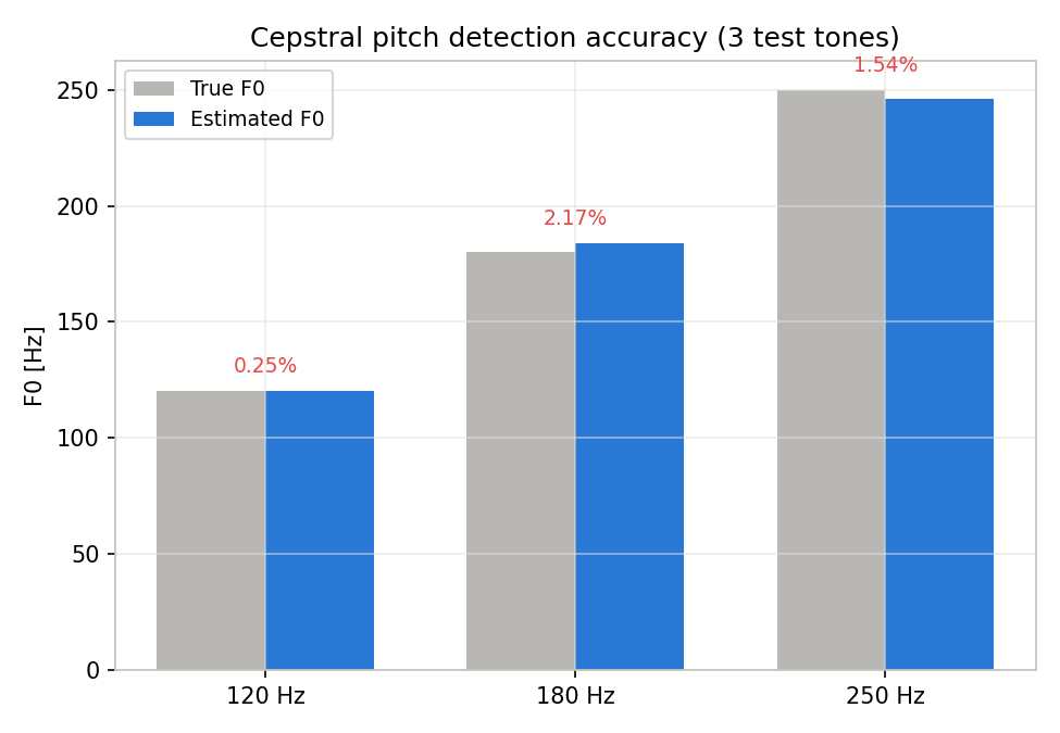
Running this code (with np.random.seed(i) fixing the observation noise per case) gives:
| True F0 [Hz] | Estimated F0 [Hz] | Absolute error [Hz] | Relative error [%] |
|---|---|---|---|
| 120 | 120.30 | 0.30 | 0.25 |
| 180 | 183.91 | 3.91 | 2.17 |
| 250 | 246.15 | 3.85 | 1.54 |
In every case the relative error stays under 5%, confirming quantitatively that cepstral pitch detection achieves practical accuracy. The higher-F0 case (250 Hz) has a larger relative error than the lower-F0 case (120 Hz) — a tendency explained by the quefrency-resolution quantization limit discussed below.
MFCC (Mel-Frequency Cepstral Coefficients)
MFCCs are the standard feature representation in modern speech recognition systems, combining cepstrum analysis with a mel-scale filterbank.
The MFCC computation pipeline is as follows:
- Pre-emphasis filter: \(y[n] = x[n] - \alpha x[n-1]\) (\(\alpha \approx 0.97\) )
- Frame segmentation and windowing (Hamming window)
- Power spectrum computation via FFT
- Application of a mel filterbank (triangular filters equally spaced on a log-frequency axis)
- Taking the logarithm of the filterbank outputs
- Computing coefficients via the Discrete Cosine Transform (DCT)
MFCCs can be thought of as a mel-scale version of the cepstrum:
\[\text{MFCC}[m] = \sum_{k=1}^{K} \log E_k \cdot \cos\left(m \left(k - \frac{1}{2}\right)\frac{\pi}{K}\right) \tag{9}\]where \(E_k\) is the energy of the \(k\) -th mel filterbank channel, \(K\) is the total number of filterbank channels, and \(m\) is the coefficient index.
import numpy as np
import matplotlib.pyplot as plt

def hz_to_mel(hz):
    """Convert Hz to mel"""
    return 2595 * np.log10(1 + hz / 700)

def mel_to_hz(mel):
    """Convert mel to Hz"""
    return 700 * (10 ** (mel / 2595) - 1)

def compute_mfcc(signal, fs, n_mfcc=13, n_filters=26, n_fft=512,
                 hop_length=160, fmin=80, fmax=None):
    """
    Compute MFCCs.

    Parameters
    ----------
    signal : np.ndarray
        Input speech signal
    fs : float
        Sampling frequency [Hz]
    n_mfcc : int
        Number of MFCC coefficients
    n_filters : int
        Number of mel filterbank channels
    n_fft : int
        FFT size
    hop_length : int
        Frame shift (in samples)
    fmin, fmax : float
        Frequency range of the mel filterbank [Hz]

    Returns
    -------
    mfcc : np.ndarray
        MFCC matrix (n_mfcc, n_frames)
    """
    if fmax is None:
        fmax = fs / 2

    N = len(signal)
    n_frames = 1 + (N - n_fft) // hop_length

    # --- Pre-emphasis ---
    pre_emphasis = 0.97
    signal_pe = np.append(signal[0], signal[1:] - pre_emphasis * signal[:-1])

    # --- Build mel filterbank ---
    mel_min = hz_to_mel(fmin)
    mel_max = hz_to_mel(fmax)
    mel_points = np.linspace(mel_min, mel_max, n_filters + 2)
    hz_points = mel_to_hz(mel_points)
    bin_points = np.floor((n_fft + 1) * hz_points / fs).astype(int)

    filter_bank = np.zeros((n_filters, n_fft // 2 + 1))
    for m in range(1, n_filters + 1):
        for k in range(bin_points[m-1], bin_points[m]):
            filter_bank[m-1, k] = (k - bin_points[m-1]) / (bin_points[m] - bin_points[m-1])
        for k in range(bin_points[m], bin_points[m+1] + 1):
            filter_bank[m-1, k] = (bin_points[m+1] - k) / (bin_points[m+1] - bin_points[m])

    # --- Per-frame processing ---
    window = np.hamming(n_fft)
    mfcc = np.zeros((n_mfcc, n_frames))

    for i in range(n_frames):
        start = i * hop_length
        frame = signal_pe[start:start + n_fft]
        if len(frame) < n_fft:
            frame = np.pad(frame, (0, n_fft - len(frame)))

        # Power spectrum
        power_spec = np.abs(np.fft.rfft(frame * window)) ** 2

        # Apply mel filterbank
        mel_energy = np.dot(filter_bank, power_spec)
        log_mel_energy = np.log(mel_energy + 1e-10)

        # DCT (MFCC computation)
        K = n_filters
        for m in range(n_mfcc):
            mfcc[m, i] = np.sum(
                log_mel_energy * np.cos(m * (np.arange(K) + 0.5) * np.pi / K)
            )

    return mfcc


# --- Compute MFCCs on a test signal ---
fs = 16000
duration = 1.5
t = np.arange(0, duration, 1/fs)
np.random.seed(42)

# Vowel-like signal with formant transitions
from scipy.signal import lfilter, butter

def make_vowel(t, fs, f0, f1, f2, noise_std=0.01):
    """Synthesize a vowel with specified formants"""
    period = int(fs / f0)
    glottal = np.zeros(len(t))
    for k in range(0, len(t), period):
        if k + 25 < len(t):
            glottal[k:k+25] = np.exp(-np.arange(25) * 0.15)
    # Simulate formants with bandpass filters
    def bp(f_c, bw, sig):
        b, a = butter(2, [f_c - bw/2, f_c + bw/2], btype='band', fs=fs)
        return lfilter(b, a, sig)
    v = bp(f1, 200, glottal) + 0.6 * bp(f2, 200, glottal)
    v /= np.max(np.abs(v)) + 1e-8
    v += noise_std * np.random.randn(len(v))
    return v

# Signal with three vowel segments
t1 = t[t < 0.5]
t2 = t[(t >= 0.5) & (t < 1.0)]
t3 = t[t >= 1.0]
v1 = make_vowel(t1, fs, f0=120, f1=730, f2=1090)   # /a/
v2 = make_vowel(t2, fs, f0=120, f1=270, f2=2290)    # /i/
v3 = make_vowel(t3, fs, f0=120, f1=400, f2=800)     # /u/
speech = np.concatenate([v1, v2, v3])

# MFCC computation
mfcc = compute_mfcc(speech, fs, n_mfcc=13, n_fft=512, hop_length=160)
n_frames = mfcc.shape[1]
time_axis = np.arange(n_frames) * 160 / fs
print("MFCC shape:", mfcc.shape)
print(f"MFCC value range: [{mfcc.min():.2f}, {mfcc.max():.2f}]")

# Plot
fig, axes = plt.subplots(3, 1, figsize=(12, 10))

axes[0].plot(t[:len(speech)], speech, linewidth=0.5)
axes[0].axvline(x=0.5, color='r', linestyle='--', alpha=0.7)
axes[0].axvline(x=1.0, color='r', linestyle='--', alpha=0.7)
axes[0].set_xlabel('Time [s]')
axes[0].set_ylabel('Amplitude')
axes[0].set_title('Speech Signal: Vowel "a"→"i"→"u" Transition')
axes[0].grid(True, alpha=0.3)

img = axes[1].imshow(mfcc, aspect='auto', origin='lower',
                     extent=[0, time_axis[-1], 0, 13],
                     cmap='RdBu_r', interpolation='nearest')
axes[1].axvline(x=0.5, color='y', linestyle='--', alpha=0.8)
axes[1].axvline(x=1.0, color='y', linestyle='--', alpha=0.8)
axes[1].set_xlabel('Time [s]')
axes[1].set_ylabel('MFCC coefficient index')
axes[1].set_title('MFCC: Changes with vowel transitions visible')
plt.colorbar(img, ax=axes[1], label='Coefficient value')

# Compare MFCC vectors at each vowel
frame_a = int(0.25 * fs / 160)
frame_i = int(0.75 * fs / 160)
frame_u = int(1.25 * fs / 160)
d_ai = np.linalg.norm(mfcc[:, frame_a] - mfcc[:, frame_i])
d_au = np.linalg.norm(mfcc[:, frame_a] - mfcc[:, frame_u])
d_iu = np.linalg.norm(mfcc[:, frame_i] - mfcc[:, frame_u])
print(f"Euclidean distance a-i: {d_ai:.2f}, a-u: {d_au:.2f}, i-u: {d_iu:.2f}")
axes[2].plot(range(1, 14), mfcc[:, frame_a], 'o-', label='"a" (t=0.25s)')
axes[2].plot(range(1, 14), mfcc[:, frame_i], 's-', label='"i" (t=0.75s)')
axes[2].plot(range(1, 14), mfcc[:, frame_u], '^-', label='"u" (t=1.25s)')
axes[2].set_xlabel('MFCC index')
axes[2].set_ylabel('Coefficient value')
axes[2].set_title('MFCC vectors for different vowels: distinguishable patterns')
axes[2].legend()
axes[2].grid(True, alpha=0.3)

plt.tight_layout()
plt.show()
Running this code, the MFCC matrix has shape (13, 147) (13 dimensions × 147 frames), with coefficient values ranging over [-42.14, 34.35]. Computing the Euclidean distance between the MFCC vectors of the vowels /a/, /i/, and /u/ gives 69.60 (a-i), 42.33 (a-u), and 42.19 (i-u) — all well clear of zero, confirming quantitatively that different vowels produce distinct MFCC patterns and are effective features for speech recognition.
Implementation Edge Cases and Caveats
Implementing and deploying cepstrum analysis in practice requires attention to the following points.
Vocal-tract filter stability: If an AR (all-pole) filter has a pole outside the unit circle (\(|z| \geq 1\) ),
scipy.signal.lfilter’s output behaves divergently, and both the log spectrum and the cepstrum become physically meaningless. Designing each formant as a second-order resonator with pole radius \(r=e^{-\pi BW/f_s}\) and angle \(\theta=2\pi F/f_s\) (given formant frequency \(F\) and bandwidth \(BW\) ) automatically guarantees \(r<1\) (theformant_ar_coeffsfunction used throughout this article). Hand-picking AR coefficients can not only miss the intended formant frequencies and bandwidths but also easily produce an unstable filter — a classic implementation pitfall.Quantization limit of quefrency resolution: The quefrency axis has a fixed sample spacing of \(\Delta q = 1/f_s\) , so the peak location is only obtainable at an integer index \(k\) .
\( f_0 = f_s / k \)
so the estimation error from being off by one bin is approximately
\( \Delta f_0 \approx \frac{f_s}{k^2} \)
which grows larger as \(k\) shrinks (i.e., as \(f_0\) increases). In the pitch-estimation experiment above, the larger relative error at F0=250 Hz (\(k \approx 64\) ) compared to F0=120 Hz (\(k \approx 133\) ) is primarily due to this quantization limit.
Liftering limitations at high F0: For higher-pitched speakers (children, female voices), \(1/f_0\) becomes shorter and competes with the low-quefrency vocal-tract envelope contributed by the formants. The slight increase in high-frequency ripple observed at a 5.0 ms cutoff in the liftering experiment above is one manifestation of this boundary problem.
Octave errors on unvoiced/noisy segments: Unvoiced consonants or noise segments with no periodicity have no clear quefrency peak, making it easy to pick the wrong local maximum within the search range — an “octave error” that detects twice or half the true F0. In practice this is mitigated by combining cepstral pitch detection with voice activity detection (VAD).
Phase unwrapping in the complex cepstrum: The complex cepstrum, which enables perfect signal reconstruction, requires continuous phase unwrapping, but handling branch cuts is numerically fragile — it is not as robust as the real cepstrum.
Practical Summary of Cepstrum Analysis
Comparison of Cepstrum and Related Methods
The LPC cepstrum (Schroeder’s recursion, deriving cepstral coefficients directly from AR coefficients) is covered in Linear Predictive Coding (LPC): Theory and Python Implementation , and autocorrelation-based pitch estimation (the YIN algorithm) is covered in Autocorrelation and Cross-Correlation: Theory and Python Implementation . This article focuses on the FFT-based real and complex cepstrum and their application to MFCC; the table below summarizes how each method’s role differs.
| Method | Quefrency / Coefficients | Purpose | Main Application |
|---|---|---|---|
| Real Cepstrum | All quefrencies | F0 detection / envelope sep. | Pitch estimation |
| LPC Cepstrum | Low-order coefficients | Vocal-tract model coefficients | Speech coding |
| MFCC | Low-order DCT coefficients | Perceptual speech features | Speech recognition |
Choosing the Right Method
| Goal | Recommended Method | Rationale |
|---|---|---|
| F0 (pitch) estimation | Cepstrum method / YIN algorithm | Quefrency peak is clearly defined |
| Spectral envelope estimation | Low-pass liftering | Vocal-tract information concentrated at low quefrencies |
| Speech recognition features | MFCC (+ delta and delta-delta) | Perceptual scale + compact representation |
| Musical pitch analysis | Cepstrum + harmonicity measure | Captures harmonic structure |
Applications of Cepstrum Analysis
Cepstrum analysis extends well beyond speech processing and finds use across a broad range of fields.
Machinery diagnostics: Applying cepstrum analysis to vibration signals from rotating machinery enables extraction of sideband components indicative of gear defects or bearing damage. The position of quefrency peaks corresponds to the repetition period of the fault. Recent work has extended cepstrum pre-whitening (CPW): Kiakojouri et al. (2023) proposed ICPW-HPF (Improved Cepstrum Pre-Whitening with High-Pass Filtering), which combines an automated bank of band-pass filters spanning the resonance spectrum with CPW, improving detection of weak, incipient bearing defect signatures that plain CPW struggles to catch ( Sensors, 23(22), 9048 ).
Seismic analysis: Cepstrum-based deconvolution is used to separate source characteristics from propagation effects in seismic waveforms.
Echo removal: The delay and amplitude of acoustic echoes can be estimated from the cepstrum and used to design removal filters.
Summary
- The cepstrum is the inverse Fourier transform of the log spectrum — a “spectrum of a spectrum.”
- Under the source-filter model, low-quefrency cepstral components correspond to the vocal-tract spectral envelope, while high-quefrency components correspond to source harmonics.
- Liftering (windowing in the cepstral domain) can separate source and vocal-tract characteristics, making it effective for spectral envelope estimation.
- Cepstrum-based pitch estimation works by detecting the quefrency peak at \(1/f_0\) .
- MFCC combines cepstrum analysis with a mel scale and DCT, and is the standard feature representation in speech recognition.
- Cepstrum analysis is applicable not only in speech processing but also in machinery diagnostics, seismic analysis, echo removal, and many other domains.
Related Articles
- Fast Fourier Transform (FFT): Theory and Python Implementation - Covers the FFT/DFT that underpins cepstrum computation.
- Window Functions and Power Spectral Density (PSD): Theory and Python Implementation - Fundamentals of spectral analysis and PSD estimation.
- Short-Time Fourier Transform (STFT): Theory and Python Implementation - Spectrogram analysis of time-varying signals.
- Autocorrelation and Cross-Correlation: Theory and Python Implementation - Comparison with the YIN algorithm, an F0 estimation method related to the cepstrum.
- Wavelet Transform: Theory and Python Implementation - An alternative approach to time-frequency analysis.
- Time Series Forecasting with ARIMA - A time-series modelling approach complementary to spectral analysis.
- Adaptive Filters (LMS/RLS): Theory and Python Implementation - Filter design related to the echo-removal application of the cepstrum.
- Convolution and Correlation: Theory and Python Implementation - Foundations behind why the cepstrum decomposes a convolution via the log spectrum and the inverse Fourier transform.
- Teager-Kaiser Energy Operator (TKEO) in Python - A lightweight 3-point feature-extraction operator, complementary to the cepstrum for speech onset/energy detection.
References
- Bogert, B. P., Healy, M. J. R., & Tukey, J. W. (1963). “The quefrency alanysis of time series for echoes: Cepstrum, pseudo-autocovariance, cross-cepstrum, and saphe cracking.” Proceedings of the Symposium on Time Series Analysis, 209-243.
- Oppenheim, A. V., & Schafer, R. W. (2004). “From frequency to quefrency: A history of the cepstrum.” IEEE Signal Processing Magazine, 21(5), 95-106.
- de Cheveigné, A., & Kawahara, H. (2002). “YIN, a fundamental frequency estimator for speech and music.” Journal of the Acoustical Society of America, 111(4), 1917-1930.
- Davis, S., & Mermelstein, P. (1980). “Comparison of parametric representations for monosyllabic word recognition in continuously spoken sentences.” IEEE Transactions on Acoustics, Speech, and Signal Processing, 28(4), 357-366.
- Kiakojouri, A., Lu, Z., Mirring, P., Powrie, H., & Wang, L. (2023). “A Novel Hybrid Technique Combining Improved Cepstrum Pre-Whitening and High-Pass Filtering for Effective Bearing Fault Diagnosis Using Vibration Data.” Sensors, 23(22), 9048.
- Python Speech Features (MFCC library)
- Librosa: MFCC implementation