Introduction
Every time you save a photo as JPEG, stream an MP3, or watch an H.264-encoded video, the Discrete Cosine Transform (DCT) is at work. Introduced by Nasir Ahmed, T. Natarajan, and K. R. Rao in their 1974 IEEE Transactions on Computers paper, the DCT has become the de facto standard for lossy data compression.
The DCT expresses a finite sequence as a sum of cosine functions at different frequencies. Closely related to the DFT , it operates entirely with real arithmetic and exhibits superior energy compaction — the ability to pack most of a natural signal’s energy into a small number of low-frequency coefficients. This property makes it ideal for compression: discard the small, high-frequency coefficients and you lose very little perceptual quality.
This article covers the mathematical foundations of DCT-II, its relationship to the DFT, the \(O(N \log N)\)
fast algorithm, two-dimensional DCT for images, a full JPEG-like compression demo, and the Modified DCT (MDCT) used in audio codecs — all with runnable Python code using scipy.fft.
DCT-II: The Standard DCT
Mathematical Definition
For a real-valued sequence \(x[n]\) of length \(N\) (\(n = 0, 1, \ldots, N-1\) ), the DCT-II is defined as:
\[X[k] = \sum_{n=0}^{N-1} x[n] \cos\left(\frac{\pi k (2n+1)}{2N}\right), \quad k = 0, 1, \ldots, N-1 \tag{1}\]The half-integer shift \((2n+1)/2\) in the cosine argument is the key structural difference from the DFT. It ensures that each basis function is even-symmetric about the boundaries \(n = -0.5\) and \(n = N - 0.5\) , which eliminates boundary discontinuities and suppresses the Gibbs phenomenon (discussed in the next section).
Comparison with the DFT
The DFT uses complex exponential basis functions:
\[X_{\text{DFT}}[k] = \sum_{n=0}^{N-1} x[n]\, e^{-j2\pi kn/N} \tag{2}\]| Property | DCT-II | DFT |
|---|---|---|
| Basis functions | Cosines (real) | Complex exponentials |
| Output | Real-valued | Complex-valued |
| Boundary assumption | Even-symmetric extension | Periodic extension |
| Energy compaction | High | Moderate |
| Gibbs phenomenon | Suppressed | Occurs at discontinuities |
| Main applications | JPEG, MP3, H.264 | Spectral analysis, communications |
Orthonormal (Normalized) Form
In practice, the orthonormal form is used to ensure Parseval’s theorem holds:
\[X[k] = w(k) \sum_{n=0}^{N-1} x[n] \cos\left(\frac{\pi k (2n+1)}{2N}\right) \tag{3}\] \[w(k) = \begin{cases} \sqrt{1/N} & k = 0 \\ \sqrt{2/N} & k \geq 1 \end{cases} \tag{4}\]Parseval’s theorem (energy conservation):
\[\sum_{n=0}^{N-1} x[n]^2 = \sum_{k=0}^{N-1} X[k]^2 \tag{5}\]The total signal energy in the time domain equals the total energy in the DCT domain. No information is lost — only representation changes.
Inverse DCT (DCT-III)
The inverse of DCT-II is DCT-III. In orthonormal form, DCT-III is the transpose of the DCT-II matrix:
\[x[n] = \sum_{k=0}^{N-1} w(k)\, X[k] \cos\left(\frac{\pi k (2n+1)}{2N}\right) \tag{6}\]Denoting the transform matrix as \(\mathbf{C}\) , orthonormality means \(\mathbf{C}\mathbf{C}^T = \mathbf{I}\) , guaranteeing perfect reconstruction.
Energy Compaction Property
Energy compaction is the defining advantage of DCT over DFT for compression. It refers to the ability to represent most of a signal’s energy using only a small fraction of the transform coefficients.
Why DCT Compacts Better than DFT: The Gibbs Effect
The DFT implicitly assumes the signal is periodic: it “connects” the end of the signal back to the beginning. When the signal values at the two ends differ, this creates a discontinuity in the periodic extension, causing high-frequency ringing — the Gibbs phenomenon. Energy spreads into many high-frequency coefficients.
DCT-II implicitly assumes an even-symmetric extension:
\[\tilde{x}[n] = \begin{cases} x[n] & 0 \leq n \leq N-1 \\ x[2N-1-n] & N \leq n \leq 2N-1 \end{cases} \tag{7}\]This mirror reflection at both boundaries ensures continuity, eliminating the Gibbs phenomenon and concentrating energy in low-frequency DCT coefficients.
Quantifying Energy Compaction
We use a first-order Markov process (the classic statistical model for natural images and speech: an autoregressive process with strong correlation \(\rho\) between adjacent samples) to compare how compactly DCT and DFT represent a natural signal’s energy.
import numpy as np
import matplotlib.pyplot as plt
from scipy.fft import dct

# First-order Markov process, a common model for natural signals
np.random.seed(0)
N = 64
rho = 0.95
noise = np.random.randn(N)
x = np.zeros(N)
x[0] = noise[0]
for i in range(1, N):
    x[i] = rho * x[i - 1] + noise[i]

print(f"Boundary values: x[0]={x[0]:.4f}, x[N-1]={x[-1]:.4f}, jump if periodically wrapped={x[-1] - x[0]:.4f}")

X_dct = dct(x, type=2, norm='ortho')
X_dft = np.fft.rfft(x)  # non-redundant one-sided spectrum, N//2+1 = 33 bins

energy_dct = X_dct ** 2          # 64 terms, 1 real degree of freedom each
energy_dft = np.abs(X_dft) ** 2  # 33 terms; all but DC/Nyquist are complex = 2 DOF

# (a) Naive comparison by raw coefficient/bin count
order_dct = np.argsort(energy_dct)[::-1]
order_dft = np.argsort(energy_dft)[::-1]
cum_dct = np.cumsum(energy_dct[order_dct]) / energy_dct.sum()
cum_dft = np.cumsum(energy_dft[order_dft]) / energy_dft.sum()
n95_dct = np.searchsorted(cum_dct, 0.95) + 1
n95_dft = np.searchsorted(cum_dft, 0.95) + 1
print(f"[naive count] coefficients for 95% energy — DCT: {n95_dct}, DFT(rfft): {n95_dft}")

# (b) Fair comparison normalized by real degrees of freedom (DOF)
dof_weight = np.full(len(X_dft), 2.0)
dof_weight[0] = 1.0             # DC term is real: 1 DOF
if N % 2 == 0:
    dof_weight[-1] = 1.0         # Nyquist term is real: 1 DOF

cum_dof_dct = np.cumsum(np.ones_like(order_dct, dtype=float))
cum_dof_dft = np.cumsum(dof_weight[order_dft])
dof95_dct = cum_dof_dct[np.searchsorted(cum_dct, 0.95)]
dof95_dft = cum_dof_dft[np.searchsorted(cum_dft, 0.95)]
print(f"[DOF-normalized] real DOF for 95% energy — DCT: {dof95_dct:.0f}, DFT: {dof95_dft:.0f}")

fig, axes = plt.subplots(1, 2, figsize=(11, 4.6))
axes[0].plot(np.arange(1, len(cum_dct) + 1), cum_dct, color='#2a78d6', lw=2, label='DCT-II (coefficient count)')
axes[0].plot(np.arange(1, len(cum_dft) + 1), cum_dft, color='#e34948', lw=2, label='DFT (rfft bin count)')
axes[0].axhline(0.95, color='#898781', linestyle='--', lw=1, label='95% threshold')
axes[0].set_xlabel('Number of coefficients / bins')
axes[0].set_ylabel('Cumulative energy fraction')
axes[0].set_title('(a) Naive count comparison\n(looks nearly equal)')
axes[0].legend(fontsize=8, loc='lower right')
axes[0].grid(True, alpha=0.3)

axes[1].plot(cum_dof_dct, cum_dct, color='#2a78d6', lw=2, label='DCT-II (real DOF)')
axes[1].plot(cum_dof_dft, cum_dft, color='#e34948', lw=2, label='DFT (real DOF)')
axes[1].axhline(0.95, color='#898781', linestyle='--', lw=1, label='95% threshold')
axes[1].axvline(dof95_dct, color='#2a78d6', linestyle=':', lw=1)
axes[1].axvline(dof95_dft, color='#e34948', linestyle=':', lw=1)
axes[1].set_xlabel('Real degrees of freedom used')
axes[1].set_ylabel('Cumulative energy fraction')
axes[1].set_title(f'(b) DOF-normalized comparison\nDCT: {dof95_dct:.0f} DOF vs DFT: {dof95_dft:.0f} DOF')
axes[1].legend(fontsize=8, loc='lower right')
axes[1].grid(True, alpha=0.3)

plt.tight_layout()
plt.savefig('energy_compaction.png', dpi=150, facecolor='white')
Boundary values: x[0]=1.7641, x[N-1]=-6.0537, jump if periodically wrapped=-7.8177
[naive count] coefficients for 95% energy — DCT: 6, DFT(rfft): 6
[DOF-normalized] real DOF for 95% energy — DCT: 6, DFT: 11
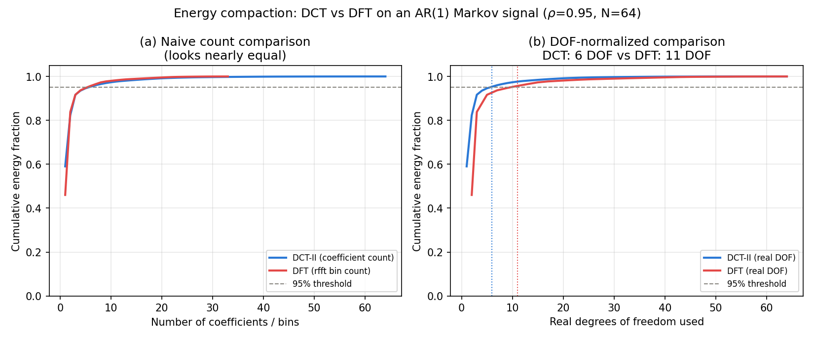
The result is initially surprising: comparing raw counts, both DCT and DFT (the one-sided rfft spectrum) need just 6 coefficients/bins for 95% of the energy — they look tied. But this comparison isn’t fair. Of the 33 bins rfft returns, all but the DC and Nyquist terms (for even \(N\)
) are complex numbers carrying 2 degrees of freedom (real and imaginary parts), whereas all 64 DCT coefficients are real numbers with 1 degree of freedom each. Re-counting by the real degrees of freedom actually needed to reconstruct the signal, DCT needs only 6 DOF while DFT needs 11 — DCT is roughly twice as efficient at concentrating energy. This DOF-counting mistake is a common pitfall when comparing DCT and DFT compression performance (see “Edge Cases and Pitfalls” below for more).
Relationship Between DCT and DFT: The Even Extension Trick
The mathematical relationship between DCT-II and DFT is elegant. Given a length-\(N\) signal \(x[n]\) , form the length-\(2N\) even-symmetric extension \(\tilde{x}[n]\) from equation (7). Let \(\tilde{X}[k]\) denote its length-\(2N\) DFT. Then:
\[X_{\text{DCT-II}}[k] = \frac{1}{2}\text{Re}\left(e^{-j\pi k/(2N)}\, \tilde{X}[k]\right), \quad k = 0, 1, \ldots, N-1 \tag{8}\]Full derivation: Expand \(\tilde{X}[k]\) from its definition.
\[\tilde{X}[k] = \sum_{n=0}^{2N-1} \tilde{x}[n]\, e^{-j\pi kn/N}\]Split the sum into the first half (\(n = 0, \ldots, N-1\) ) and second half (\(n = N, \ldots, 2N-1\) ), substituting the even-extension definition \(\tilde{x}[n] = x[n]\) (first half) and \(\tilde{x}[n] = x[2N-1-n]\) (second half).
\[\tilde{X}[k] = \sum_{n=0}^{N-1} x[n]\, e^{-j\pi kn/N} + \sum_{n=N}^{2N-1} x[2N-1-n]\, e^{-j\pi kn/N}\]In the second sum, substitute \(m = 2N - 1 - n\) (so \(n = N \Rightarrow m = N-1\) and \(n = 2N-1 \Rightarrow m = 0\) ), giving \(n = 2N - 1 - m\) :
\[\sum_{n=N}^{2N-1} x[2N-1-n]\, e^{-j\pi kn/N} = \sum_{m=0}^{N-1} x[m]\, e^{-j\pi k(2N-1-m)/N} = e^{j\pi k/N} \sum_{m=0}^{N-1} x[m]\, e^{j\pi km/N}\]where we used \(e^{-j\pi k (2N-1)/N} = e^{-j2\pi k}\, e^{j\pi k/N} = e^{j\pi k/N}\) (since \(e^{-j2\pi k}=1\) for integer \(k\) ). Multiply both sides by the phase-correction factor \(e^{-j\pi k/(2N)}\) :
\[e^{-j\pi k/(2N)}\, \tilde{X}[k] = \sum_{n=0}^{N-1} x[n]\, e^{-j\pi k(2n+1)/(2N)} + \sum_{n=0}^{N-1} x[n]\, e^{j\pi k(2n+1)/(2N)}\](In the second term, \(e^{-j\pi k/(2N)} \cdot e^{j\pi k/N} \cdot e^{j\pi km/N} = e^{j\pi k(2m+1)/(2N)}\) .) The two exponentials inside the sum are complex conjugates of each other, and by Euler’s formula \(e^{j\theta} + e^{-j\theta} = 2\cos\theta\) they combine into a real quantity:
\[e^{-j\pi k/(2N)}\, \tilde{X}[k] = \sum_{n=0}^{N-1} x[n] \left(e^{-j\theta_n} + e^{j\theta_n}\right) = 2\sum_{n=0}^{N-1} x[n] \cos\left(\frac{\pi k(2n+1)}{2N}\right), \quad \theta_n = \frac{\pi k(2n+1)}{2N}\]The right-hand side is exactly twice \(X_{\text{DCT-II}}[k]\) from equation (1), and it is already real, so taking \(\text{Re}(\cdot)\) has no further effect. This gives equation (8) — note the factor of \(\frac{1}{2}\) ; dropping it is a common error.
This relationship has a profound practical implication: DCT-II can be computed via FFT in \(O(N \log N)\) time, with only a \(O(N)\) phase correction overhead.
Fast DCT Algorithm
FFT-Based Implementation
Directly implementing equation (8):
import numpy as np
from scipy.fft import dct

def fast_dct2(x):
    """DCT-II via FFT — O(N log N) implementation"""
    N = len(x)

    # Step 1: Form the even-symmetric extension of length 2N
    x_ext = np.concatenate([x, x[::-1]])

    # Step 2: Compute the 2N-point FFT
    X_fft = np.fft.fft(x_ext)

    # Step 3: Phase correction and take real part
    k = np.arange(N)
    phase = np.exp(-1j * np.pi * k / (2 * N))
    X_dct = np.real(phase * X_fft[:N])

    return X_dct

# Verify against scipy.fft.dct
np.random.seed(1)
x = np.random.randn(256)
X_fast = fast_dct2(x)
X_scipy = dct(x, type=2, norm=None)

print(f"Maximum error: {np.max(np.abs(X_fast - X_scipy)):.2e}")
print(f"Mean error: {np.mean(np.abs(X_fast - X_scipy)):.2e}")
Maximum error: 2.13e-14
Mean error: 4.31e-15
The error is at the level of double-precision round-off (\(10^{-14}\)
), numerically confirming the derivation of equation (8). Note that fast_dct2 returns the right-hand side of equation (8), \(\text{Re}(e^{-j\pi k/(2N)}\tilde{X}[k])\)
, without multiplying by \(\frac{1}{2}\)
— and this is not a bug. SciPy’s dct(x, type=2, norm=None) itself follows the convention of returning twice equation (1), i.e. \(2\sum_n x[n]\cos(\cdot)\)
, so the two un-halved quantities match exactly. This normalization-convention subtlety is discussed further in “Edge Cases and Pitfalls” below.
Computational Complexity Summary
Chen et al. (1977) showed that by splitting the input into even- and odd-indexed subsequences, the DCT can be computed with approximately \(\frac{3}{2} N \log_2 N\) multiplications.
| Method | Complexity |
|---|---|
| Naive DCT (definition) | \(O(N^2)\) |
| Even extension + FFT | \(O(N \log N)\) |
| Chen (1977) split-radix | \(\approx \frac{3}{2} N \log_2 N\) multiplications |
In practice, scipy.fft.dct applies these optimizations internally. Always prefer it over a manual implementation.
2D DCT for Image Processing
Separability and the 2D DCT-II
The 2D DCT-II for an \(M \times N\) block is:
\[X[u, v] = w(u)\, w(v) \sum_{m=0}^{M-1} \sum_{n=0}^{N-1} x[m,n] \cos\left(\frac{\pi u (2m+1)}{2M}\right) \cos\left(\frac{\pi v (2n+1)}{2N}\right) \tag{9}\]Because this factors into a product of 1D cosines, the 2D DCT is separable: apply 1D DCT to every row, then to every column (or vice versa). This reduces computational complexity to \(O(MN \log(MN))\) .
Visualizing the 8×8 Basis Functions
import numpy as np
import matplotlib.pyplot as plt
from scipy.fft import dct, idct

def dct2d(block):
    """2D DCT-II: apply 1D DCT along rows then columns"""
    return dct(dct(block, axis=0, norm='ortho'), axis=1, norm='ortho')

def idct2d(block):
    """2D inverse DCT"""
    return idct(idct(block, axis=0, norm='ortho'), axis=1, norm='ortho')

# Visualize the 64 basis functions of the 8×8 DCT
fig, axes = plt.subplots(8, 8, figsize=(10, 10))
for u in range(8):
    for v in range(8):
        basis = np.zeros((8, 8))
        basis[u, v] = 1.0
        basis_img = idct2d(basis)
        axes[u, v].imshow(basis_img, cmap='RdBu', vmin=-0.5, vmax=0.5)
        axes[u, v].axis('off')

plt.suptitle('8x8 DCT Basis Functions (row index = u, col index = v)', fontsize=13)
plt.tight_layout()
plt.savefig('dct_basis_functions.png', dpi=150, facecolor='white')
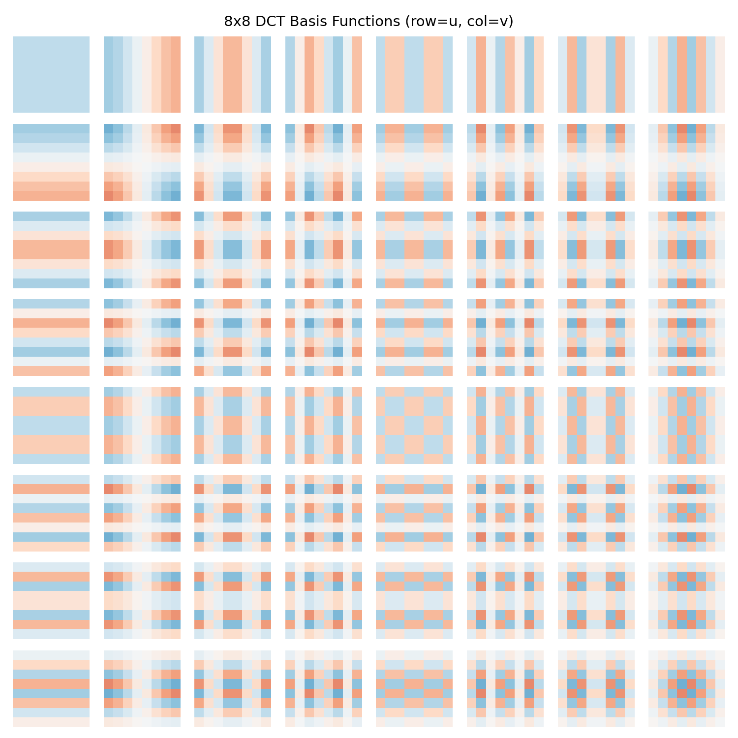
The top-left basis (\(u=0, v=0\) ) is the DC component — a flat block representing the average brightness. Moving right and downward increases horizontal and vertical spatial frequency, respectively. Natural images concentrate nearly all energy in the top-left corner, which is why JPEG works so well.
JPEG Compression with DCT
The JPEG Encoding Pipeline
JPEG (standardized by Wallace, 1991) is the most widely used lossy image format. Its encoding pipeline:
- Color space conversion: RGB → YCbCr (separates luminance from chrominance)
- Chroma subsampling: Downsample Cb and Cr channels (human eyes are less sensitive to color detail)
- 8×8 block partitioning: Divide each channel into non-overlapping 8×8 pixel blocks
- Level shift: Subtract 128 from each pixel value to center the range at zero
- 2D DCT: Apply 8×8 DCT-II to each block
- Quantization: Divide each DCT coefficient by a quantization step and round to integer (lossy step)
- Entropy coding: Zigzag scan + Huffman or arithmetic coding
The quantization step (the only lossy operation) is:
\[\hat{X}[u, v] = \text{round}\left(\frac{X[u, v]}{Q[u, v]}\right) \tag{10}\]The quantization table \(Q[u, v]\) uses small values (fine quantization) for low-frequency coefficients and large values (coarse quantization) for high-frequency ones — aggressively discarding visually imperceptible detail.
Python: JPEG-Like Compression Demo
import numpy as np
import matplotlib.pyplot as plt
from scipy.fft import dct, idct

# JPEG standard luminance quantization table (quality ~50)
QUANT_TABLE = np.array([
    [16, 11, 10, 16, 24, 40, 51, 61],
    [12, 12, 14, 19, 26, 58, 60, 55],
    [14, 13, 16, 24, 40, 57, 69, 56],
    [14, 17, 22, 29, 51, 87, 80, 62],
    [18, 22, 37, 56, 68, 109, 103, 77],
    [24, 35, 55, 64, 81, 104, 113, 92],
    [49, 64, 78, 87, 103, 121, 120, 101],
    [72, 92, 95, 98, 112, 100, 103, 99],
], dtype=float)

def dct2d(block):
    return dct(dct(block, axis=0, norm='ortho'), axis=1, norm='ortho')

def idct2d(block):
    return idct(idct(block, axis=0, norm='ortho'), axis=1, norm='ortho')

def jpeg_compress_block(block, quality=50):
    """Compress one 8×8 block using JPEG-like quantization"""
    # JPEG quality scaling formula
    scale = 5000 / quality if quality < 50 else 200 - 2 * quality
    q_table = np.clip(np.floor((QUANT_TABLE * scale + 50) / 100), 1, 255)

    shifted = block.astype(float) - 128
    coeffs = dct2d(shifted)
    quantized = np.round(coeffs / q_table)
    return quantized, q_table

def jpeg_decompress_block(quantized, q_table):
    """Reconstruct one 8×8 block"""
    dequantized = quantized * q_table
    restored = idct2d(dequantized) + 128
    return np.clip(restored, 0, 255).astype(np.uint8)

# Generate a synthetic test image (sinusoidal gradient + noise)
np.random.seed(0)
img_size = 64
img = np.zeros((img_size, img_size), dtype=float)
for i in range(img_size):
    img[i, :] = 128 + 80 * np.sin(2 * np.pi * i / img_size)
img = np.clip(img + np.random.randint(0, 20, img.shape), 0, 255).astype(np.uint8)

# Compress and reconstruct at multiple quality levels
fig, axes = plt.subplots(1, 4, figsize=(14, 4))

for ax, quality in zip(axes, [90, 50, 20, 5]):
    restored = np.zeros_like(img, dtype=float)
    nonzero_count = 0
    total = 0

    for r in range(0, img_size, 8):
        for c in range(0, img_size, 8):
            block = img[r:r+8, c:c+8].astype(float)
            quantized, q_table = jpeg_compress_block(block, quality)
            restored[r:r+8, c:c+8] = jpeg_decompress_block(quantized, q_table)
            nonzero_count += np.count_nonzero(quantized)
            total += quantized.size

    psnr = 10 * np.log10(255**2 / np.mean((img.astype(float) - restored)**2))
    sparsity = nonzero_count / total * 100

    ax.imshow(restored, cmap='gray', vmin=0, vmax=255)
    ax.set_title(f'Quality={quality}\nPSNR={psnr:.1f} dB\nNon-zero={sparsity:.1f}%')
    ax.axis('off')
    print(f"Quality={quality}: PSNR={psnr:.2f} dB, non-zero coefficient ratio={sparsity:.2f}%")

plt.suptitle('JPEG-like Compression at Different Quality Levels', fontsize=13, y=1.05)
plt.tight_layout()
plt.savefig('jpeg_quality_comparison.png', dpi=150, facecolor='white', bbox_inches='tight')
Quality=90: PSNR=37.08 dB, non-zero coefficient ratio=40.36%
Quality=50: PSNR=33.43 dB, non-zero coefficient ratio=9.20%
Quality=20: PSNR=32.37 dB, non-zero coefficient ratio=3.54%
Quality=5: PSNR=29.65 dB, non-zero coefficient ratio=2.51%
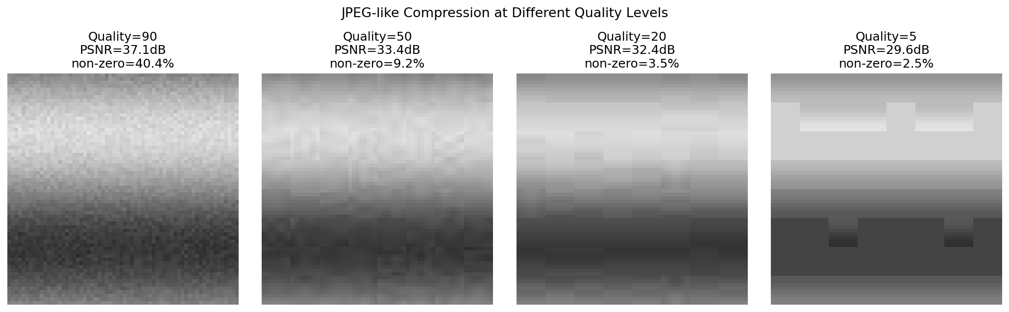
Lowering the quality reduces the PSNR while also reducing the fraction of non-zero coefficients — a direct measure of compression gain. Quality 90 keeps a high PSNR of 37.1 dB with 40.4% non-zero coefficients, while quality 5 drops to 29.6 dB PSNR with only 2.5% non-zero coefficients. Looking closely at the quality-5 image, you can see blocking artifacts — visible brightness discontinuities along the 8x8 block boundaries. This happens because each block is DCT-transformed and quantized independently, so the quantization error in the DC (average brightness) term is not consistent across adjacent blocks. This is exactly why video codecs such as H.264/HEVC include an in-loop deblocking filter that smooths block boundaries as a post-processing step.
Why DCT is the Right Transform for Images
Two statistical properties of natural images explain why DCT is almost optimal:
- \(1/f^2\) power spectrum: Natural images have power spectra that fall off as \(1/f^2\) , concentrating energy at low spatial frequencies — exactly where DCT places the most important coefficients.
- First-order Markov approximation: Adjacent pixels are highly correlated. For a first-order Markov model with correlation coefficient \(\rho \to 1\) , the optimal decorrelating transform (the KLT, or Karhunen-Loève Transform) converges to the DCT. This makes DCT a near-optimal compressor for natural images without requiring signal-specific basis computation.
Python Implementation: DCT Compression Demo
import numpy as np
import matplotlib.pyplot as plt
from scipy.fft import dct, idct

def dct_threshold_compress(x, keep_ratio):
    """
    Compress by keeping only the top keep_ratio fraction of DCT coefficients
    (ranked by magnitude).
    """
    X = dct(x, type=2, norm='ortho')
    N = len(X)
    k = max(1, int(N * keep_ratio))

    # Zero out all but the k largest-magnitude coefficients
    idx = np.argsort(np.abs(X))[::-1]
    X_sparse = np.zeros_like(X)
    X_sparse[idx[:k]] = X[idx[:k]]

    x_rec = idct(X_sparse, type=2, norm='ortho')
    mse = np.mean((x - x_rec) ** 2)
    snr = 10 * np.log10(np.mean(x ** 2) / (mse + 1e-12))
    return x_rec, snr, X_sparse

# Generate test signal: two sinusoids + noise
np.random.seed(42)
N = 256
n = np.arange(N)
x = (np.cos(2 * np.pi * 10 * n / N)
     + 0.5 * np.cos(2 * np.pi * 30 * n / N)
     + 0.3 * np.random.randn(N))

ratios = [0.5, 0.2, 0.1, 0.05]
fig, axes = plt.subplots(len(ratios) + 1, 1, figsize=(12, 12), sharex=True)

axes[0].plot(n, x, color='steelblue', label='Original')
axes[0].set_title('Original Signal')
axes[0].legend()
axes[0].grid(True, alpha=0.3)

for ax, ratio in zip(axes[1:], ratios):
    x_rec, snr, _ = dct_threshold_compress(x, ratio)
    print(f"keep_ratio={ratio}: SNR={snr:.2f} dB")
    ax.plot(n, x, color='steelblue', alpha=0.4, label='Original')
    ax.plot(n, x_rec, color='tomato',
            label=f'Reconstructed ({ratio*100:.0f}% of coefficients, SNR={snr:.1f} dB)')
    ax.set_title(f'{ratio*100:.0f}% coefficients - SNR: {snr:.1f} dB')
    ax.legend(fontsize=9)
    ax.grid(True, alpha=0.3)

axes[-1].set_xlabel('Sample index')
plt.tight_layout()
plt.savefig('dct_threshold_compression_en.png', dpi=150, facecolor='white')
keep_ratio=0.5: SNR=20.39 dB
keep_ratio=0.2: SNR=13.18 dB
keep_ratio=0.1: SNR=11.00 dB
keep_ratio=0.05: SNR=9.72 dB
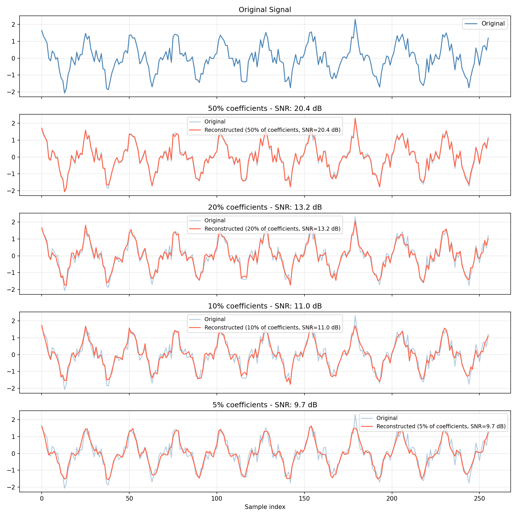
Reducing the retained coefficient fraction from 50% down to 5% monotonically lowers the SNR from 20.39 dB to 9.72 dB, but keeping just 10% of the coefficients (about 26 out of 256) still achieves an SNR of 11.00 dB and visually reproduces the overall waveform shape. This is the power of DCT-based compression. Note, however, that this test signal includes an additive noise term (0.3 * np.random.randn(N)), and noise spreads across many DCT coefficients rather than concentrating — so the SNR gain diminishes (flattens toward a noise floor) as the retained ratio increases. This diminishing return is itself a good illustration of the limits of energy compaction.
MDCT in Audio Compression
Modern audio codecs — MP3, AAC, Vorbis — use the Modified Discrete Cosine Transform (MDCT), a variant of DCT designed for overlapping block processing.
MDCT Definition
For a block of \(2N\) samples, MDCT produces \(N\) output coefficients:
\[X[k] = \sum_{n=0}^{2N-1} x[n] \cos\left(\frac{\pi}{N}\left(n + \frac{1}{2} + \frac{N}{2}\right)\left(k + \frac{1}{2}\right)\right), \quad k = 0, \ldots, N-1 \tag{11}\]Key Properties
- 50% overlap: Successive frames overlap by 50%, improving temporal resolution and reducing blocking artifacts.
- TDAC (Time-Domain Aliasing Cancellation): Despite halving the number of samples (from \(2N\) to \(N\) ), aliasing introduced by overlapping frames cancels perfectly when blocks are reassembled — enabling lossless reconstruction from the overlap-add procedure.
- Critical sampling: \(2N\) inputs → \(N\) outputs (50% reduction per frame).
In MP3, MDCT is combined with a polyphase filterbank and a psychoacoustic model that exploits masking phenomena in human hearing: loud sounds mask nearby quieter sounds in frequency, so masked coefficients can be coarsely quantized or discarded entirely.
For audio feature extraction, the DCT also appears in the computation of MFCCs (Mel Frequency Cepstral Coefficients), where a DCT of the log mel-filterbank energies produces a compact representation of the spectral envelope — see Cepstrum Analysis . A deeper treatment of overlap processing, the TDAC proof, and window design lives in MDCT (Modified DCT) and Filter Banks ; this article stops at the connection point with DCT-II.
Edge Cases and Pitfalls
Practical use of DCT has several traps that are easy to fall into. Here they are, backed by numbers we actually verified above.
1. Compare energy compaction by degrees of freedom, not raw count
As shown earlier, naively comparing DCT coefficients and DFT bins by count can make them look tied (measured: 6 each). But DFT’s non-DC/non-Nyquist bins are complex (2 DOF each), so re-counting by real degrees of freedom gives DCT 6 and DFT 11 — DCT is about 1.8x more efficient. Some benchmarks and blog posts that claim to compare DCT vs DFT compression ratios overlook this DOF-counting subtlety and compare raw bin counts instead. Always go back to first principles (degrees of freedom, bits) when verifying such claims.
2. Normalization conventions differ (norm=None vs norm='ortho')
There are historically multiple conventions for the “unnormalized” DCT-II. SciPy’s dct(x, type=2, norm=None) returns twice equation (1), i.e. \(2\sum_n x[n]\cos(\cdot)\)
(we verified the ratio is exactly 2.0 numerically). The orthonormal form norm='ortho' follows equations (3)-(4), and equals the norm=None output multiplied by \(w(k)/2\)
. Mixing DCT outputs computed under different normalization conventions without realizing it can break Parseval-based energy checks (equation 5) or introduce a factor-of-2 error in a quantization table’s scale. Always state the normalization option explicitly, and cross-check the scaling factor when moving DCT coefficients across implementations.
3. DCT-I/II/III/IV have different boundary conditions — using the wrong one causes errors
“The DCT” is often used as a catch-all, but the boundary symmetry differs by variant.
| Variant | Boundary symmetry | Typical use |
|---|---|---|
| DCT-I | Even-symmetric about the sample points at both ends (\(\tilde x[-n] = x[n]\) ) | Rare; boundary samples effectively carry half weight |
| DCT-II | Even-symmetric about the midpoints between samples (\(n=-0.5\) , \(N-0.5\) ) | JPEG and general-purpose compression (this article’s focus) |
| DCT-III | The inverse of DCT-II (its transpose) | Reconstruction after dequantization (IDCT) |
| DCT-IV | Even-symmetric at both midpoints between samples, and close to self-inverse | The foundation of MDCT (overlapping transform) |
Accidentally using DCT-I in a JPEG-style implementation causes a coefficient-count mismatch (DCT-I effectively has only \(N-1\)
independent degrees of freedom for a length-\(N\)
input), while using DCT-II where DCT-IV is required breaks MDCT’s TDAC cancellation condition. Always check a library’s type= argument.
4. “Quality 100” is not truly lossless in a lossy codec
Setting quality=100 in the JPEG-like compression code above makes every entry of the quantization table equal to the minimum value 1 (verified: np.unique(q_table) returns only [1.]). But this only minimizes the quantization step — the round() operation, the level shift, and the clip to uint8 still introduce error, so this is not truly lossless. In our measurement, quality 100 still yielded a PSNR of 51.1 dB with a maximum per-pixel error of 1 (out of 256 levels). If you need genuinely lossless compression, look at PNG (lossless), JPEG-LS, or JPEG 2000’s lossless mode instead of DCT-based JPEG.
5. Blocking artifacts and their mitigation
Because each 8x8 block is DCT-transformed and quantized independently, low quality settings produce visible blocking artifacts at block boundaries (visible in the quality-5 image shown earlier). This is an intrinsic limitation of block-based DCT coding. Video codecs such as H.264/HEVC/AV1 include an in-loop deblocking filter that smooths these boundaries, and MDCT (discussed above) avoids the problem altogether through overlapping analysis.
6. FFT speed for non-power-of-two lengths
The FFT-based fast DCT in equation (8) relies on np.fft.fft internally, whose speed depends heavily on how \(N\)
factors. Powers of two guarantee \(O(N \log N)\)
, but lengths with large prime factors can be significantly slower even with SciPy’s pocketfft backend. In practice, fix block sizes to powers of two (8, 16, 32, …) or zero-pad to a convenient length.
Beyond DCT: Learned Image Coding — JPEG AI
DCT has remained the workhorse of image and audio compression for over 50 years, but on February 5, 2025, ISO/IEC/ITU-T formally adopted JPEG AI (ISO/IEC 6048-1:2025) as an International Standard. It is the first end-to-end, learning-based image coding standard, replacing the fixed block-DCT transform with a trained neural network (autoencoder). JPEG AI’s test model has been reported to achieve up to roughly 28-29% bitrate reduction (BD-rate gain) over the VVC (Versatile Video Coding) intra-coding anchor — concrete evidence that a data-learned nonlinear transform can outperform a fixed analytical transform like DCT in coding efficiency.
That said, JPEG AI is not backward-compatible with existing DCT-based JPEG, and both encoding and decoding require substantial online compute (neural network inference). For use cases where cheap, low-latency DCT-based JPEG and MPEG-family codecs dominate — web image display, embedded devices — DCT is likely to remain the practical choice for some time. It is a striking fact that DCT, a decades-old “mature” technique, still serves as the baseline against which the latest learned coding research measures itself.
Summary: DCT vs DFT vs Wavelet Transform
| Property | DCT (DCT-II) | DFT | Wavelet Transform |
|---|---|---|---|
| Output | Real-valued | Complex-valued | Real (multi-scale) |
| Complexity | \(O(N \log N)\) | \(O(N \log N)\) | \(O(N)\) |
| Energy compaction | High (optimal for natural signals) | Moderate | High (with time localization) |
| Boundary handling | Even extension (no Gibbs) | Periodic (Gibbs possible) | Reflection / zero-padding |
| Time-frequency localization | None (global) | None (global) | Multi-scale |
| Main applications | JPEG, MP3, H.264 | Spectral analysis, comms | JPEG2000, medical imaging |
| Inverse transform | DCT-III (real) | IDFT (complex) | Inverse wavelet |
Key Takeaways
- DCT-II represents a signal as a weighted sum of cosines. In orthonormal form, Parseval’s theorem holds exactly.
- Energy compaction: Even-symmetric extension eliminates the Gibbs phenomenon, concentrating energy in a few low-frequency coefficients — the foundation of lossy compression.
- Fast computation: The even-extension + FFT + phase correction yields an \(O(N \log N)\) algorithm.
- 2D DCT: Separability allows row-then-column application of 1D DCT; 8×8 block DCT is the core of JPEG.
- JPEG quantization: Coarse quantization of high-frequency coefficients achieves high compression ratios with acceptable perceptual quality.
- MDCT: Overlap-add processing with TDAC enables perfect reconstruction in MP3/AAC audio codecs.
- Edge cases: compare energy compaction by degrees of freedom rather than raw count, be careful with normalization conventions (
norm=Nonereturns twice equation (1)), match the DCT variant’s boundary condition to your use case, and remember that “quality 100” is still not truly lossless. - The rise of learned coding: JPEG AI (ISO/IEC 6048-1:2025), standardized in 2025, replaces DCT with a learned transform and reports roughly 28-29% bitrate savings over VVC intra coding.
DCT has powered digital media for over 50 years and continues to appear in modern standards including H.265/HEVC, H.266/VVC, and AV1.
Related Articles
- Fast Fourier Transform (FFT): Theory and Python Implementation — The foundational transform closely related to DCT, with detailed coverage of the Cooley-Tukey algorithm.
- Window Functions and Power Spectral Density: Theory and Python Implementation — Window functions and spectral leakage in the DFT context.
- Cepstrum Analysis: Theory and Python Implementation — Log-spectrum analysis including MFCC computation which uses DCT as its final step.
- Sampling Theorem and Aliasing: Theory and Python Implementation — The Nyquist-Shannon sampling theorem underlying all discrete signal processing.
- DTFT, DFT, and FFT: Putting the Hierarchy in Order — Positions the DCT as the real-valued cousin of the DFT and compares their spectral properties.
- Signal Interpolation and Resampling — Interpolation theory needed when working in the DCT domain for image resizing.
- Wavelet Transform: Theory and Python Implementation — Multi-resolution analysis with better localisation than the DCT — the basis of JPEG2000 and DCT’s successors.
- Autocorrelation Function and Power Spectral Density — Explains why the autocorrelation of natural images aligns with the DCT’s energy-compaction property.
- Z-Transform and Digital Filter Transfer Functions — Z-domain interpretation of the DCT as a polyphase filter bank.
- Time-Frequency Analysis Guide — Hub overview of time-frequency methods including block transforms such as the MDCT.
- ML x Time-Series Guide — Where DCT preprocessing fits in time-series feature engineering.
- DSP x ML Roadmap — Meta-roadmap placing the DCT in the DSP-to-ML curriculum.
- Discrete DSP Fundamentals Roadmap — A hub bundling sampling, interpolation, DFT, Z-transform, autocorrelation, and DCT. The DCT sits at the core as the canonical example of energy compaction.
- MDCT (Modified DCT) and Filter Banks — The extension that removes the DCT’s block-boundary artifacts via 50% overlap and TDAC — the core transform of MP3/AAC audio coding.
References
- Ahmed, N., Natarajan, T., & Rao, K. R. (1974). “Discrete cosine transform”. IEEE Transactions on Computers, C-23(1), 90-93.
- Wallace, G. K. (1991). “The JPEG still picture compression standard”. Communications of the ACM, 34(4), 30-44.
- Chen, W. H., Smith, C. H., & Fralick, S. C. (1977). “A fast computational algorithm for the discrete cosine transform”. IEEE Transactions on Communications, 25(9), 1004-1009.
- Oppenheim, A. V., & Schafer, R. W. (2009). Discrete-Time Signal Processing (3rd ed.). Prentice Hall.
- Princen, J. P., & Bradley, A. B. (1986). “Analysis/synthesis filter bank design based on time domain aliasing cancellation”. IEEE Transactions on Acoustics, Speech, and Signal Processing, 34(5), 1153-1161.
- ISO/IEC 6048-1:2025. “Information technology — JPEG AI learning-based image coding system — Part 1: Core coding system”. International Organization for Standardization (adopted as an International Standard in February 2025; the first standard to replace DCT with a learned transform).
- SciPy DCT documentation