Introduction
When performing spectral analysis with the Fast Fourier Transform (FFT) , the result is commonly displayed as a magnitude spectrum showing how much power each frequency component carries. However, the Fourier transform output is complex-valued, and alongside the magnitude it encodes a phase spectrum that is equally important yet frequently overlooked.
Why does phase matter in practice?
Consider applying a Butterworth filter to a speech or biomedical signal. Even when the magnitude response is nearly ideal, the filtered waveform can exhibit visible distortion — transients spread out, sharp edges become blurred, and the temporal relationships between frequency components are altered. This distortion arises entirely from the filter’s nonlinear phase response: different frequency components are delayed by different amounts as they pass through the filter. The quantity that captures this frequency-dependent delay is the group delay.
This article provides a systematic treatment of phase spectrum and group delay: their mathematical definitions, the physical interpretation of group delay as signal travel time, the linear phase property of
FIR filters
, the nonlinear phase distortion inherent to IIR filters, and the use of all-pass filters for phase equalization — all illustrated with Python implementations using scipy.signal.
Phase Spectrum: Definition and Properties
Complex Frequency Response and Phase
The frequency response of a discrete-time linear filter evaluated on the unit circle is:
\[H(e^{j\omega}) = |H(e^{j\omega})| \cdot e^{j\phi(\omega)} \tag{1}\]where \(\omega \in [0, \pi]\) is the normalized angular frequency (\(\omega = \pi\) corresponds to the Nyquist frequency), and:
- \(|H(e^{j\omega})|\) — magnitude response: the gain applied to each frequency component
- \(\phi(\omega) = \angle H(e^{j\omega})\) — phase response: the phase shift imparted to each frequency component
The phase response is computed as:
\[\phi(\omega) = \arctan\left(\frac{\mathrm{Im}[H(e^{j\omega})]}{\mathrm{Re}[H(e^{j\omega})]}\right) \tag{2}\]Wrapped vs. Unwrapped Phase
Because \(\arctan\) has range \((-\pi, \pi]\) , the directly computed phase is wrapped: it exhibits artificial \(\pm\pi\) discontinuities even when the true underlying phase varies continuously. For instance, a continuously decreasing phase may appear as \(-3.10 \to -3.14 \to 3.12 \to 3.10\) , with a \(2\pi\) jump at the boundary.
The unwrapped phase removes these discontinuities by adding the appropriate integer multiples of \(2\pi\) :
\[\phi_{\mathrm{unwrap}}(\omega) = \phi(\omega) + 2\pi \, k(\omega), \quad k(\omega) \in \mathbb{Z} \tag{3}\]In Python, np.unwrap() performs this operation automatically. Unwrapped phase is essential for meaningful group delay computation, since numerical differentiation of the wrapped phase produces large spurious spikes at each \(2\pi\)
discontinuity.
Linear Phase and Nonlinear Phase
The most significant distinction in filter phase behavior is between linear phase and nonlinear phase.
A filter has linear phase if:
\[\phi(\omega) = -\omega \cdot \tau_0 \tag{4}\]where \(\tau_0\) is a constant called the phase delay. In this case, every frequency component is shifted by a phase proportional to its frequency — which is mathematically equivalent to a pure time delay of \(\tau_0\) samples. The output waveform is an exact replica of the input, shifted in time.
A filter has nonlinear phase when \(\phi(\omega)\) deviates from a straight line. In this case, the delay experienced by each frequency component differs, and a waveform composed of multiple frequencies will emerge distorted.
Group Delay: Definition and Physical Interpretation
Mathematical Definition
The group delay is defined as the negative derivative of the phase response with respect to angular frequency:
\[\tau_g(\omega) = -\frac{d\phi(\omega)}{d\omega} \tag{5}\]Group delay has units of samples (or seconds when multiplied by the sampling period \(T_s = 1/f_s\) ). When \(\tau_g(\omega) = \tau_0\) (constant), the filter has linear phase. When \(\tau_g(\omega)\) varies with \(\omega\) , the filter has nonlinear phase and introduces group delay distortion.
Substituting the linear phase condition \(\phi(\omega) = -\omega \tau_0\) into equation \((5)\) confirms:
\[\tau_g(\omega) = -\frac{d(-\omega \tau_0)}{d\omega} = \tau_0 \tag{6}\]Physical Interpretation: Envelope Delay
The physical meaning of group delay becomes clear by examining a narrowband signal — a slowly modulated carrier:
\[x(t) = a(t)\cos(\omega_0 t)\]where \(a(t)\) is the slowly varying envelope and \(\omega_0\) is the carrier frequency. After passing through a filter \(H\) , the output is approximately:
\[y(t) \approx |H(e^{j\omega_0})| \cdot a(t - \tau_g(\omega_0)) \cdot \cos(\omega_0 t - \phi(\omega_0)) \tag{7}\]The envelope \(a(t)\) is delayed by the group delay \(\tau_g(\omega_0)\) , while the carrier is phase-shifted by \(\phi(\omega_0)\) . Thus, the group delay quantifies how many samples (or seconds) a signal packet centered at frequency \(\omega_0\) is delayed by the filter.
If group delay is frequency-independent (linear phase), all signal packets arrive at the output simultaneously and the waveform is preserved. If group delay varies with frequency (group delay distortion), different frequency bands arrive at different times, causing the output waveform to be stretched, smeared, or distorted relative to the input.
Consequences of Group Delay Distortion
Group delay distortion causes problems in many practical applications:
- Waveform distortion: A square wave contains harmonics at odd multiples of the fundamental. If high harmonics are delayed more than the fundamental (or vice versa), the reconstructed waveform loses its sharp edges.
- Biomedical signal processing: In ECG analysis, the shape of the QRS complex is diagnostically significant. Phase distortion can alter the morphology of these transient waveforms, potentially affecting automated detection algorithms.
- Audio systems: Group delay variations across the audio band cause audible coloration — transients lose crispness, and the perceived spatial localization of sounds may shift.
- Digital communications: In bandlimited channels, frequency-dependent group delay causes inter-symbol interference (ISI), spreading each transmitted symbol into adjacent time slots.
- Feedback control: In closed-loop systems, group delay constitutes a frequency-dependent phase lag that erodes phase margin and can destabilize the loop.
Linear Phase FIR Filters
Why Symmetric Coefficients Guarantee Linear Phase
An \(N\) -tap FIR filter with impulse response \(h[n]\) has transfer function:
\[H(z) = \sum_{n=0}^{N-1} h[n] z^{-n} \tag{8}\]If the coefficients satisfy the even symmetry condition:
\[h[n] = h[N-1-n], \quad n = 0, 1, \ldots, N-1 \tag{9}\]then the frequency response can be factored as:
\[H(e^{j\omega}) = e^{-j\omega(N-1)/2} \cdot A(\omega) \tag{10}\]where \(A(\omega)\) is a real-valued amplitude function. This factorization shows that the phase response is:
\[\phi(\omega) = -\frac{N-1}{2}\omega + \begin{cases} 0 & \text{if } A(\omega) > 0 \\ \pi & \text{if } A(\omega) < 0 \end{cases} \tag{11}\]In the passband where \(A(\omega) > 0\) , the phase is exactly linear: \(\phi(\omega) = -\frac{N-1}{2}\omega\) . The group delay is therefore constant:
\[\tau_g = \frac{N-1}{2} \quad \text{[samples]} \tag{12}\]A key insight is that the group delay equals half the filter length minus one. A 65-tap FIR filter introduces a fixed delay of 32 samples at all frequencies within the passband — a pure time shift, with no waveform distortion.
The Four Types of Linear Phase FIR Filters
Linear phase FIR filters are classified into four types based on coefficient symmetry and filter length parity:
| Type | Symmetry | Length | Applicable filter types | Constraint |
|---|---|---|---|---|
| I | Even: \(h[n] = h[N-1-n]\) | Odd | Lowpass, highpass, bandpass | None (most general) |
| II | Even: \(h[n] = h[N-1-n]\) | Even | Lowpass | \(H(\pi) = 0\) (cannot be highpass) |
| III | Odd: \(h[n] = -h[N-1-n]\) | Odd | Differentiator, Hilbert | \(H(0) = H(\pi) = 0\) |
| IV | Odd: \(h[n] = -h[N-1-n]\) | Even | Highpass, differentiator | \(H(0) = 0\) |
Type I is the most commonly used for general-purpose filtering. scipy.signal.firwin produces Type I or II filters depending on whether the specified number of taps is odd or even.
Zero-Phase Filtering for Offline Processing
The constant group delay of a linear phase FIR filter is \(\frac{N-1}{2}\) samples — a non-zero delay. In offline processing where causality is not required, this delay can be eliminated entirely using forward-backward filtering:
- Filter the signal in the forward direction to obtain \(y_1[n]\)
- Reverse \(y_1[n]\)
- Filter again in the forward direction, then reverse again
The net result has zero phase shift and a squared magnitude response:
\[H_{\text{zero-phase}}(e^{j\omega}) = |H(e^{j\omega})|^2 \tag{13}\]scipy.signal.filtfilt implements this procedure. It doubles the effective filter order and cannot be used for real-time (causal) processing, but it completely eliminates phase distortion.
Nonlinear Phase in IIR Filters
Why IIR Filters Cannot Achieve Linear Phase
An IIR filter with rational transfer function:
\[H(z) = \frac{B(z)}{A(z)} = \frac{\sum_{k=0}^{M} b_k z^{-k}}{1 + \sum_{k=1}^{N} a_k z^{-k}} \tag{14}\]has poles located inside the unit circle. The phase response of \(H(e^{j\omega})\) can be decomposed as a sum of contributions from each zero and pole:
\[\phi(\omega) = \sum_k \angle(e^{j\omega} - z_k) - \sum_k \angle(e^{j\omega} - p_k) \tag{15}\]where \(z_k\) and \(p_k\) are the zeros and poles respectively. Since the poles are located asymmetrically relative to the unit circle (they are inside it, with no mirror-image poles outside), the phase response is generally a nonlinear function of \(\omega\) . This is a fundamental property of stable IIR filters — it cannot be circumvented by choice of filter coefficients.
Group Delay Comparison of Classical IIR Filters
The following table summarizes the group delay characteristics of classical IIR filter designs:
| Filter | Transition bandwidth | Passband group delay | Primary use case |
|---|---|---|---|
| Butterworth | Moderate | Relatively smooth | General-purpose, moderate phase |
| Chebyshev Type I | Narrow | More distorted | Amplitude-critical applications |
| Chebyshev Type II | Narrow | Moderate | Stopband attenuation priority |
| Elliptic (Cauer) | Narrowest | Most distorted | Minimum-order design |
| Bessel | Wide | Maximally flat | Waveform preservation priority |
The Bessel filter is designed with the explicit objective of maximizing the flatness of group delay in the passband (Maximally Flat Group Delay criterion). It achieves the best time-domain waveform fidelity among IIR filters, at the cost of a very gradual transition between passband and stopband.
The Fundamental Trade-off
The relationship between magnitude sharpness and group delay flatness represents a fundamental trade-off in IIR filter design:
- Sharper amplitude transition → more poles clustered near the unit circle in the transition region → larger group delay variation
- Flatter group delay → poles more evenly distributed → gentler amplitude roll-off
When both sharp magnitude cutoff and flat group delay are required simultaneously, the only general solution is to use an IIR filter for amplitude shaping followed by an all-pass filter for phase equalization.
All-Pass Filters for Phase Equalization
Definition and Transfer Function
An all-pass filter (APF) has unit magnitude response at all frequencies:
\[|H_{AP}(e^{j\omega})| = 1, \quad \forall \omega \tag{16}\]while its phase response — and therefore its group delay — can be freely shaped by choice of pole/zero locations. The first-order all-pass filter transfer function is:
\[H_{AP}^{(1)}(z) = \frac{z^{-1} - a}{1 - az^{-1}}, \quad |a| < 1 \tag{17}\]This filter has a zero at \(z = 1/a\) (outside the unit circle) and a pole at \(z = a\) (inside the unit circle), placed in a mirror-image relationship with respect to the unit circle. This mirror-image placement ensures that the magnitude response is identically 1 for all \(\omega\) .
For a complex pole at \(z = re^{j\theta}\) (\(r < 1\) ), the all-pass filter and its complex conjugate are combined into a second-order real-coefficient all-pass filter:
\[H_{AP}(z) = \frac{z^{-1} - a^*}{1 - az^{-1}} \tag{18}\]The practical second-order implementation with real coefficients is:
\[H_{AP}^{(2)}(z) = \frac{r^2 - 2r\cos\theta \cdot z^{-1} + z^{-2}}{1 - 2r\cos\theta \cdot z^{-1} + r^2 z^{-2}} \tag{19}\]Phase and Group Delay of the First-Order All-Pass Filter
For the first-order all-pass filter with real coefficient \(a\) (\(0 < a < 1\) ), the phase response is:
\[\phi_{AP}(\omega) = -\omega - 2\arctan\left(\frac{a\sin\omega}{1 - a\cos\omega}\right) \tag{20}\]The group delay is:
\[\tau_g^{AP}(\omega) = \frac{1 - a^2}{1 - 2a\cos\omega + a^2} \tag{21}\]This is always positive (the all-pass filter only adds delay, never advances the signal), and exhibits a peak near \(\omega = 0\) . For the second-order filter, the peak is located near \(\omega = \theta\) (the angle of the pole), and its height is controlled by \(r\) (the pole radius). A value of \(r\) close to 1 produces a sharp, tall peak; a smaller \(r\) gives a broad, low peak.
Group Delay Equalization Strategy
Phase equalization using all-pass filters follows this procedure:
- Measure the group delay \(\tau_g^{\text{target}}(\omega)\)
of the IIR filter to be equalized using
scipy.signal.group_delay. - Identify the frequency regions where \(\tau_g^{\text{target}}(\omega)\) is smallest relative to the maximum — these are the regions where additional delay needs to be added.
- Design all-pass sections (choosing \(r\) and \(\theta\) for each second-order section) to add delay in these regions, bringing the total group delay closer to a flat response.
- Cascade the all-pass sections after the original IIR filter.
Since \(|H_{AP}| = 1\) , the amplitude response of the original filter is preserved exactly. The equalization is imperfect in general (particularly at the passband edge), but significant improvement is achievable with a few all-pass sections.
Research context: group delay equalization remains an active research area. Zhang et al. (2025) propose an alternative to discrete-time all-pass equalization: a microwave bandpass filter equalized with a defected-ground-structure (DGS) negative group delay (NGD) circuit, which cancels the positive group delay peak that appears at the passband edges. Their third-order prototype reduced measured group delay ripple from 0.55 ns to 0.25 ns, a 54.5% reduction (Zhang et al., “A group delay equalization method for filters based on DGS NGD structure,” Electromagnetics, 2025). Although implemented in continuous-time microwave circuits rather than discrete-time all-pass sections, the underlying principle is the same one demonstrated numerically below: cancel a filter’s group-delay imbalance by adding a compensating element with an opposing group-delay profile.
Python Implementation
Setup: Library Imports
import numpy as np
import matplotlib.pyplot as plt
from scipy.signal import butter, sosfilt, freqz, firwin, group_delay, lfilter, iirfilter
from scipy.signal import cheby1, ellip, bessel
Phase Response: Wrapped vs. Unwrapped
# --- Filter design ---
fs = 1000          # sampling frequency [Hz]
fc = 100           # cutoff frequency [Hz]
N_iir = 8          # IIR filter order
N_fir = 64         # FIR filter tap count

# Butterworth IIR filter (ba form)
b_iir, a_iir = butter(N_iir, fc, fs=fs, output='ba')

# Linear-phase FIR filter (Hamming window)
b_fir = firwin(N_fir, fc, fs=fs, window='hamming')
a_fir = np.array([1.0])

# --- Frequency response ---
worN = 4096
w, H_iir = freqz(b_iir, a_iir, worN=worN, fs=fs)
_, H_fir = freqz(b_fir, a_fir, worN=worN, fs=fs)

# --- Phase computation ---
phase_iir_wrapped = np.angle(H_iir)          # wrapped phase
phase_iir = np.unwrap(np.angle(H_iir))       # unwrapped phase
phase_fir = np.unwrap(np.angle(H_fir))       # FIR (linear phase)

# --- Plot ---
fig, axes = plt.subplots(3, 1, figsize=(10, 10))

# Magnitude
axes[0].plot(w, 20 * np.log10(np.abs(H_iir) + 1e-12),
             label=f'IIR Butterworth N={N_iir}')
axes[0].plot(w, 20 * np.log10(np.abs(H_fir) + 1e-12),
             label=f'FIR Hamming {N_fir} taps', linestyle='--')
axes[0].set_xlabel('Frequency [Hz]')
axes[0].set_ylabel('Magnitude [dB]')
axes[0].set_title('Magnitude Response')
axes[0].set_xlim(0, fs / 2)
axes[0].set_ylim(-80, 5)
axes[0].axvline(fc, color='gray', linestyle=':', alpha=0.5, label='Cutoff')
axes[0].legend()
axes[0].grid(True, alpha=0.3)

# Wrapped vs unwrapped phase (IIR)
axes[1].plot(w, np.degrees(phase_iir_wrapped),
             label='IIR (wrapped)', color='orange')
axes[1].plot(w, np.degrees(phase_iir),
             label='IIR (unwrapped)', color='blue')
axes[1].set_xlabel('Frequency [Hz]')
axes[1].set_ylabel('Phase [degrees]')
axes[1].set_title('Phase Response: Wrapped vs Unwrapped (IIR Butterworth)')
axes[1].set_xlim(0, fs / 2)
axes[1].legend()
axes[1].grid(True, alpha=0.3)

# IIR vs FIR phase
axes[2].plot(w, np.degrees(phase_iir),
             label=f'IIR Butterworth N={N_iir} (nonlinear)')
axes[2].plot(w, np.degrees(phase_fir),
             label=f'FIR Hamming {N_fir} taps (linear)', linestyle='--')
axes[2].set_xlabel('Frequency [Hz]')
axes[2].set_ylabel('Phase [degrees]')
axes[2].set_title('Phase Response: IIR vs FIR')
axes[2].set_xlim(0, fs / 2)
axes[2].legend()
axes[2].grid(True, alpha=0.3)

plt.tight_layout()
plt.savefig('phase_response_comparison.png')

# --- Verify wrapping: count discontinuities where |Δφ| > 0.9π ---
wrap_jumps = np.sum(np.abs(np.diff(phase_iir_wrapped)) > np.pi * 0.9)
print(f"Number of wrapped-phase discontinuities: {wrap_jumps}")
print(f"Unwrapped phase range: {np.degrees(phase_iir.max()):.2f} deg to {np.degrees(phase_iir.min()):.2f} deg")
Output:
Number of wrapped-phase discontinuities: 13
Unwrapped phase range: 0.00 deg to -905.56 deg
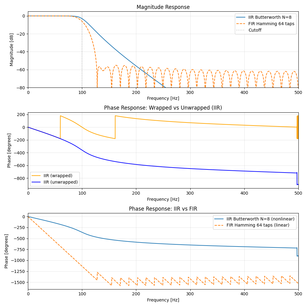
The middle panel shows the wrapped phase (orange) jumping discontinuously across \(\pm 180°\) 13 times, while the unwrapped phase (blue) decreases smoothly and monotonically. In the bottom panel, the FIR phase (green dashed) is a straight line through the origin, whereas the IIR phase (blue solid) follows a nonlinear curve that reaches roughly \(-905.6°\) near the Nyquist frequency — a direct numerical illustration of the qualitative difference between the two filter types.
Group Delay Calculation and Comparison
# --- Group delay via scipy.signal.group_delay ---
worN = 4096
w_gd, gd_iir = group_delay((b_iir, a_iir), w=worN, fs=fs)
w_gd, gd_fir = group_delay((b_fir, a_fir), w=worN, fs=fs)

# --- Finite difference approximation (for illustration) ---
w_arr, H_iir_arr = freqz(b_iir, a_iir, worN=worN * 2, fs=fs)
omega_arr = w_arr * 2 * np.pi / fs   # Hz → rad/sample
phase_arr = np.unwrap(np.angle(H_iir_arr))

# τ_g(ω) ≈ −Δφ/Δω
gd_diff = -np.diff(phase_arr) / np.diff(omega_arr)
w_diff = (w_arr[:-1] + w_arr[1:]) / 2   # midpoints

# --- Plot ---
fig, axes = plt.subplots(2, 1, figsize=(10, 8))

axes[0].plot(w_gd, gd_iir,
             label=f'IIR Butterworth N={N_iir}', color='blue')
axes[0].plot(w_gd, gd_fir,
             label=f'FIR Hamming {N_fir} taps (constant = {(N_fir-1)/2:.1f} samples)',
             linestyle='--', color='red')
axes[0].axhline((N_fir - 1) / 2, color='red', linestyle=':', alpha=0.5)
axes[0].set_xlabel('Frequency [Hz]')
axes[0].set_ylabel('Group Delay [samples]')
axes[0].set_title('Group Delay: IIR vs FIR')
axes[0].set_xlim(0, fs / 2)
axes[0].set_ylim(-5, 50)
axes[0].legend()
axes[0].grid(True, alpha=0.3)

axes[1].plot(w_diff, gd_diff,
             label='IIR (finite difference)', color='purple', alpha=0.7)
axes[1].plot(w_gd, gd_iir,
             label='IIR (scipy.signal.group_delay)', color='blue', linestyle='--')
axes[1].set_xlabel('Frequency [Hz]')
axes[1].set_ylabel('Group Delay [samples]')
axes[1].set_title('Group Delay: Finite Difference vs scipy.signal.group_delay')
axes[1].set_xlim(0, fs / 2)
axes[1].set_ylim(-5, 50)
axes[1].legend()
axes[1].grid(True, alpha=0.3)

plt.tight_layout()
plt.savefig('group_delay_comparison.png')

print(f"FIR group delay: min={gd_fir.min():.6f}, max={gd_fir.max():.6f}, std={gd_fir.std():.2e}")
print(f"Theoretical value (N_fir-1)/2 = {(N_fir - 1) / 2}")
mask_pb = (w_gd >= 0) & (w_gd <= 90)
print(f"IIR group delay (passband 0-90 Hz): min={gd_iir[mask_pb].min():.3f}, max={gd_iir[mask_pb].max():.3f} samples")

gd_iir_interp = np.interp(w_diff, w_gd, gd_iir)
mask_valid = (w_diff > 5) & (w_diff < fs / 2 - 5)
diff_err = np.abs(gd_diff[mask_valid] - gd_iir_interp[mask_valid])
print(f"Error between finite-difference and scipy.group_delay: mean={diff_err.mean():.4f}, max={diff_err.max():.4f} samples")
Output:
FIR group delay: min=31.499999, max=31.500002, std=3.59e-08
Theoretical value (N_fir-1)/2 = 31.5
IIR group delay (passband 0-90 Hz): min=7.888, max=14.584 samples
Error between finite-difference and scipy.group_delay: mean=0.0009, max=0.9531 samples
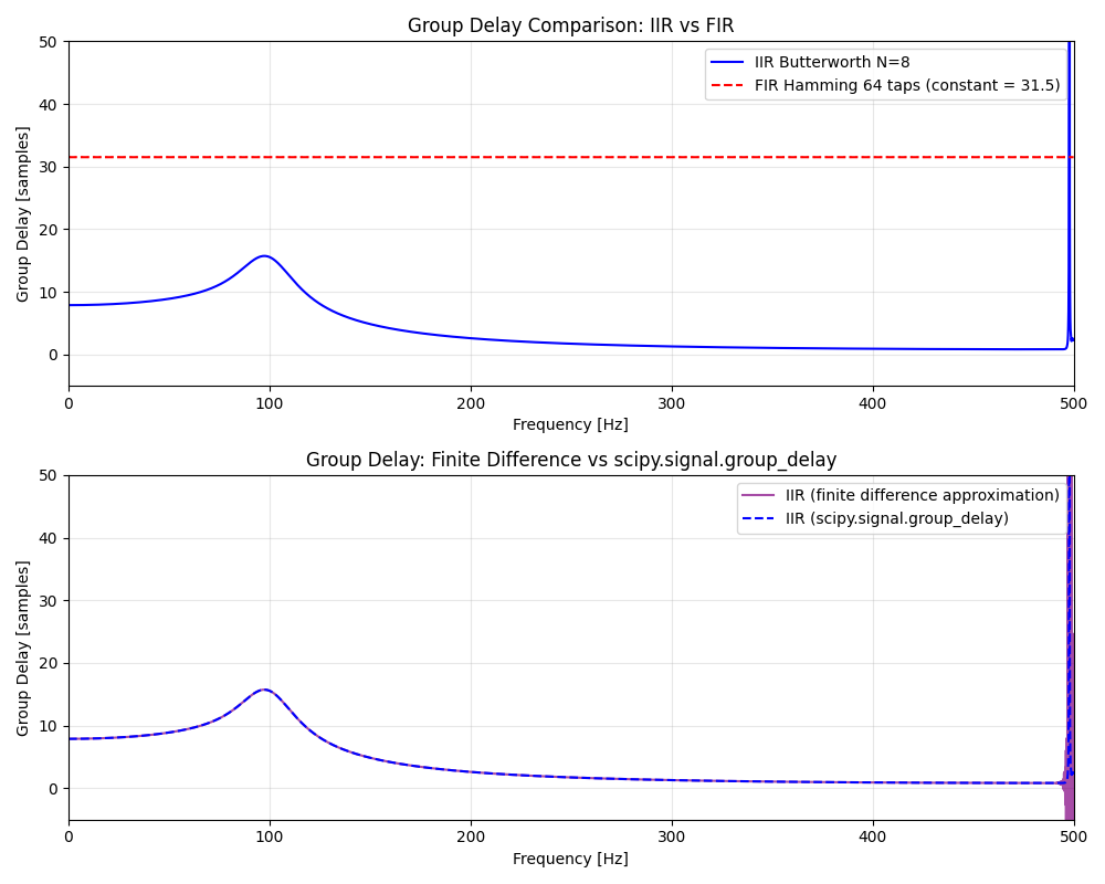
The FIR filter’s group delay matches the theoretical value \((N-1)/2 = 31.5\)
samples to within floating-point precision — a standard deviation of just \(3.59 \times 10^{-8}\)
samples — confirming equation \((12)\)
numerically. The Butterworth IIR filter’s group delay, by contrast, ranges from 7.888 to 14.584 samples over the passband alone (0-90 Hz), demonstrating clear frequency dependence. The finite-difference approximation \(-\Delta\phi/\Delta\omega\)
agrees with scipy.signal.group_delay to a mean error of just 0.0009 samples, though the maximum error grows to 0.9531 samples near the wrapped-phase discontinuities, where the unwrapping procedure accumulates numerical error.
Waveform Distortion Due to Phase Nonlinearity
# --- Test signal: sum of harmonics ---
fs = 1000
t = np.arange(0, 0.5, 1/fs)

# Multicomponent signal (10, 30, 50, 70, 90 Hz)
freqs_sig = [10, 30, 50, 70, 90]
x = sum(np.sin(2 * np.pi * f * t) / f for f in freqs_sig)

# --- Filtering ---
fc_test = 200   # high cutoff — all components pass through

# IIR Butterworth (nonlinear phase)
b_iir_t, a_iir_t = butter(6, fc_test, fs=fs, output='ba')
y_iir = lfilter(b_iir_t, a_iir_t, x)

# FIR linear-phase filter
b_fir_t = firwin(101, fc_test, fs=fs, window='hamming')
y_fir = lfilter(b_fir_t, [1.0], x)

# Compensate FIR group delay shift
fir_delay = 50   # (101 - 1) / 2 = 50 samples
y_fir_aligned = np.concatenate([y_fir[fir_delay:], np.zeros(fir_delay)])

# --- Plot ---
fig, axes = plt.subplots(3, 1, figsize=(12, 8), sharex=True)

axes[0].plot(t, x, 'k', linewidth=1.5)
axes[0].set_title('Original Signal (10 + 30 + 50 + 70 + 90 Hz)')
axes[0].set_ylabel('Amplitude')
axes[0].grid(True, alpha=0.3)

axes[1].plot(t, y_iir, color='blue')
axes[1].plot(t, x, 'k--', alpha=0.3, linewidth=1, label='Original')
axes[1].set_title('After IIR Butterworth (nonlinear phase — waveform distorted)')
axes[1].set_ylabel('Amplitude')
axes[1].legend()
axes[1].grid(True, alpha=0.3)

axes[2].plot(t, y_fir_aligned, color='red')
axes[2].plot(t, x, 'k--', alpha=0.3, linewidth=1, label='Original')
axes[2].set_title('After FIR linear-phase (delay-corrected — shape preserved)')
axes[2].set_xlabel('Time [s]')
axes[2].set_ylabel('Amplitude')
axes[2].legend()
axes[2].grid(True, alpha=0.3)

plt.tight_layout()
plt.savefig('waveform_distortion.png')

# --- Quantitative evaluation: RMSE over the mid-section, excluding transients ---
mask_mid = (t >= 0.15) & (t <= 0.35)
rmse_iir = np.sqrt(np.mean((y_iir[mask_mid] - x[mask_mid]) ** 2))
rmse_fir = np.sqrt(np.mean((y_fir_aligned[mask_mid] - x[mask_mid]) ** 2))
print(f"Agreement with original (mid-section 0.15-0.35 s, RMSE): IIR={rmse_iir:.5f}, FIR(delay-corrected)={rmse_fir:.5f}")
print(f"Signal RMS amplitude: {np.sqrt(np.mean(x[mask_mid] ** 2)):.5f}")
Output:
Agreement with original (mid-section 0.15-0.35 s, RMSE): IIR=0.02584, FIR(delay-corrected)=0.00011
Signal RMS amplitude: 0.07694
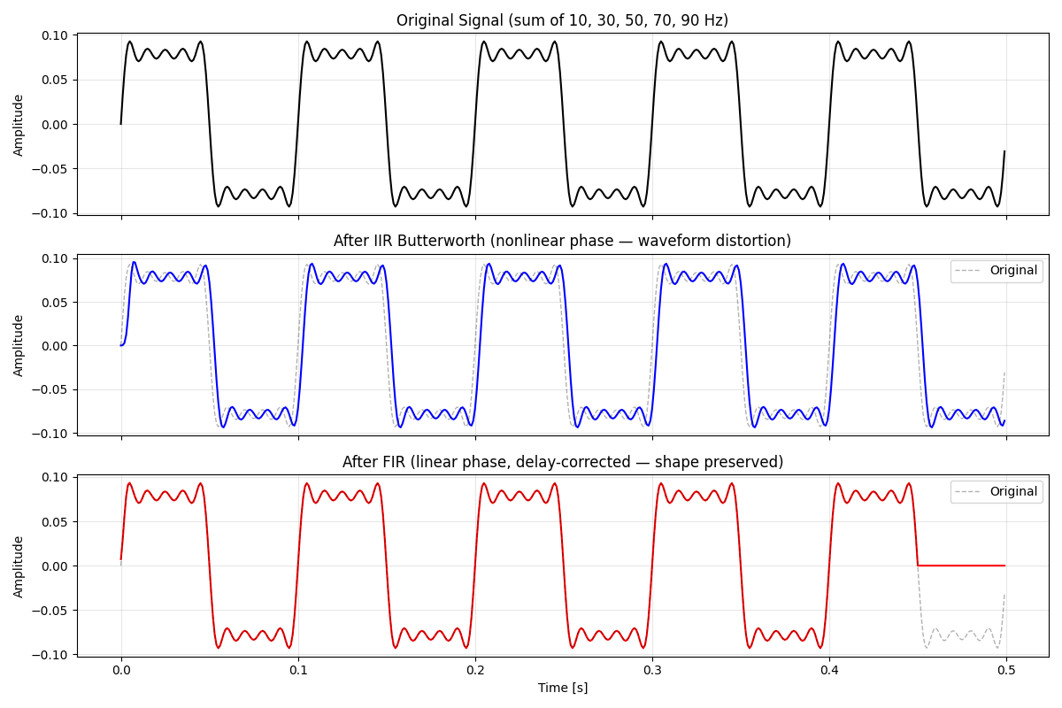
Against a signal RMS amplitude of 0.07694, the IIR Butterworth output has an RMSE of 0.02584 relative to the original (about 34% of the RMS amplitude) — a clearly distorted waveform. The delay-corrected FIR output, in contrast, has an RMSE of only 0.00011 (about 0.14% of the RMS amplitude), reproducing the original almost perfectly. This is direct numerical confirmation that a linear-phase FIR filter introduces nothing more than a pure time shift.
All-Pass Filter Design and Phase Equalization
def allpass_filter_2nd(r, theta):
    """
    Compute second-order all-pass filter coefficients.

    Transfer function:
        H_AP(z) = (r^2 - 2r*cos(θ)*z^{-1} + z^{-2})
                / (1 - 2r*cos(θ)*z^{-1} + r^2*z^{-2})

    Parameters
    ----------
    r : float
        Pole radius (0 < r < 1). Larger r → sharper group delay peak.
    theta : float
        Pole angle in radians. Controls peak frequency location.

    Returns
    -------
    b, a : ndarray
        Numerator and denominator coefficients (b = numerator, a = denominator).
    """
    c = 2 * r * np.cos(theta)
    r2 = r ** 2
    b = np.array([r2, -c, 1.0])
    a = np.array([1.0, -c, r2])
    return b, a


# --- All-pass filter characterization ---
worN = 4096
fig, axes = plt.subplots(3, 1, figsize=(10, 10))

r_values = [0.5, 0.7, 0.9]
theta_ap = np.pi / 4   # peak group delay near ω = π/4

peak_info = []
for r in r_values:
    b_ap, a_ap = allpass_filter_2nd(r, theta_ap)
    w_ap, H_ap = freqz(b_ap, a_ap, worN=worN, fs=fs)
    w_gd_ap, gd_ap = group_delay((b_ap, a_ap), w=worN, fs=fs)

    mag_db = 20 * np.log10(np.abs(H_ap) + 1e-12)
    axes[0].plot(w_ap, mag_db, label=f'r={r}')
    axes[1].plot(w_ap, np.degrees(np.unwrap(np.angle(H_ap))), label=f'r={r}')
    axes[2].plot(w_gd_ap, gd_ap, label=f'r={r}')

    peak_freq = w_gd_ap[np.argmax(gd_ap)]
    peak_info.append((r, mag_db.max(), mag_db.min(), gd_ap.max(), peak_freq))

axes[0].set_title('All-Pass Filter: Magnitude Response (must be 0 dB)')
axes[0].set_xlabel('Frequency [Hz]')
axes[0].set_ylabel('Magnitude [dB]')
axes[0].set_ylim(-3, 3)
axes[0].legend()
axes[0].grid(True, alpha=0.3)

axes[1].set_title('All-Pass Filter: Phase Response')
axes[1].set_xlabel('Frequency [Hz]')
axes[1].set_ylabel('Phase [degrees]')
axes[1].legend()
axes[1].grid(True, alpha=0.3)

axes[2].set_title('All-Pass Filter: Controllable Group Delay Peak')
axes[2].set_xlabel('Frequency [Hz]')
axes[2].set_ylabel('Group Delay [samples]')
axes[2].set_ylim(0, 30)
axes[2].legend()
axes[2].grid(True, alpha=0.3)

plt.tight_layout()
plt.savefig('allpass_response.png')

for r_v, mag_max, mag_min, gd_peak, peak_freq in peak_info:
    print(f"r={r_v}: magnitude range=[{mag_min:.2e}, {mag_max:.2e}] dB, "
          f"group delay peak={gd_peak:.3f} samples @ {peak_freq:.2f} Hz")
Output:
r=0.5: magnitude range=[8.68e-12, 8.69e-12] dB, group delay peak=3.610 samples @ 118.16 Hz
r=0.7: magnitude range=[8.68e-12, 8.69e-12] dB, group delay peak=6.010 samples @ 124.39 Hz
r=0.9: magnitude range=[8.67e-12, 8.70e-12] dB, group delay peak=19.105 samples @ 125.00 Hz
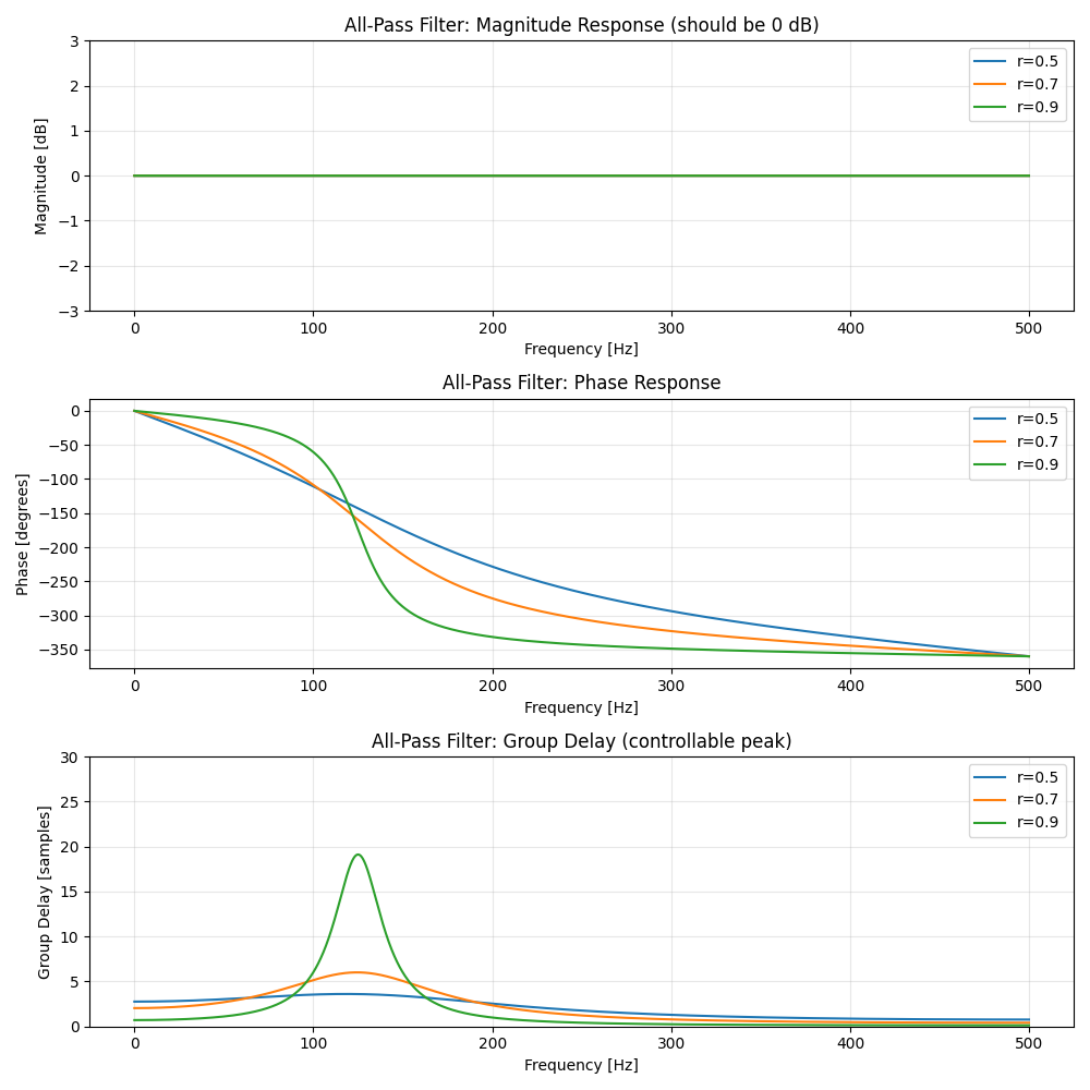
The top panel confirms that, regardless of pole radius \(r\) , the magnitude response stays at 0 dB to within numerical error (\(10^{-12}\) dB). In the bottom panel, the group delay peak grows sharply from 3.610 to 6.010 to 19.105 samples as \(r\) increases from 0.5 to 0.7 to 0.9 — numerically confirming that moving the pole closer to the unit circle produces a sharper, taller group delay peak. The peak location (roughly 118-125 Hz) matches the pole angle \(\theta_{ap} = \pi/4\) (normalized frequency) chosen in the design.
Verifying Group-Delay Equalization: Butterworth IIR + All-Pass Filter
Flattening group delay with an all-pass filter requires placing its group-delay peak in the frequency region where the target filter’s own group delay is lowest. The Butterworth IIR filter’s group delay is smallest at the low end of the passband and increases toward the cutoff (as measured above: 7.888-14.584 samples over 0-90 Hz). Placing the all-pass peaks at low frequencies raises the delay there, bringing the overall profile closer to flat.
# --- Phase equalization: Butterworth + all-pass filter ---
fs = 1000
fc = 100
N_butter = 6

b_butter, a_butter = butter(N_butter, fc, fs=fs, output='ba')
w_hz, gd_butter = group_delay((b_butter, a_butter), w=4096, fs=fs)

# Design all-pass sections to flatten the group delay:
# place the peaks in the low-frequency region, where the Butterworth
# filter's own group delay is lowest, so they raise it toward the
# passband-edge value.
r_ap = 0.5
theta_ap1 = 2 * np.pi * 5 / fs    # peak near 5 Hz
theta_ap2 = 2 * np.pi * 10 / fs   # peak near 10 Hz

b_ap1, a_ap1 = allpass_filter_2nd(r_ap, theta_ap1)
b_ap2, a_ap2 = allpass_filter_2nd(r_ap, theta_ap2)

# Cascade: convolve coefficients
b_total = np.convolve(np.convolve(b_butter, b_ap1), b_ap2)
a_total = np.convolve(np.convolve(a_butter, a_ap1), a_ap2)

w_hz, gd_total = group_delay((b_total, a_total), w=4096, fs=fs)
w_hz, gd_ap1 = group_delay((b_ap1, a_ap1), w=4096, fs=fs)
w_hz, gd_ap2 = group_delay((b_ap2, a_ap2), w=4096, fs=fs)

fig, axes = plt.subplots(2, 1, figsize=(10, 8))

# Magnitude response (all-pass sections should not affect amplitude)
w_hz_mag, H_butter = freqz(b_butter, a_butter, worN=4096, fs=fs)
_, H_total = freqz(b_total, a_total, worN=4096, fs=fs)
axes[0].plot(w_hz_mag,
             20 * np.log10(np.abs(H_butter) + 1e-12),
             label='Butterworth only', color='blue')
axes[0].plot(w_hz_mag,
             20 * np.log10(np.abs(H_total) + 1e-12),
             label='Butterworth + APF (equalized)', color='red', linestyle='--')
axes[0].set_xlabel('Frequency [Hz]')
axes[0].set_ylabel('Magnitude [dB]')
axes[0].set_title('Magnitude Response: All-Pass Equalization Preserves Amplitude')
axes[0].set_xlim(0, fs / 2)
axes[0].set_ylim(-80, 5)
axes[0].legend()
axes[0].grid(True, alpha=0.3)

# Group delay comparison
axes[1].plot(w_hz, gd_butter,
             label=f'Butterworth N={N_butter}', color='blue')
axes[1].plot(w_hz, gd_ap1 + gd_ap2,
             label='APF contribution (ap1 + ap2)', color='green', linestyle='--')
axes[1].plot(w_hz, gd_total,
             label='Butterworth + APF (equalized)', color='red', linewidth=2)
axes[1].set_xlabel('Frequency [Hz]')
axes[1].set_ylabel('Group Delay [samples]')
axes[1].set_title('Group Delay Equalization with All-Pass Filter')
axes[1].set_xlim(0, fc * 2)
axes[1].set_ylim(0, 30)
axes[1].axvline(fc, color='gray', linestyle=':', alpha=0.5, label='Cutoff')
axes[1].legend()
axes[1].grid(True, alpha=0.3)

plt.tight_layout()
plt.savefig('group_delay_equalization.png')

mask_pb = (w_hz >= 0) & (w_hz <= fc)
gd_butter_range = gd_butter[mask_pb].max() - gd_butter[mask_pb].min()
gd_total_range = gd_total[mask_pb].max() - gd_total[mask_pb].min()
mag_diff = np.abs(20 * np.log10(np.abs(H_butter) + 1e-12) - 20 * np.log10(np.abs(H_total) + 1e-12))
print(f"Passband (0-{fc} Hz) group delay spread: Butterworth only={gd_butter_range:.3f} samples, "
      f"Butterworth+APF={gd_total_range:.3f} samples")
print(f"Max magnitude difference (full band): {mag_diff.max():.6f} dB")
Output:
Passband (0-100 Hz) group delay spread: Butterworth only=4.994 samples, Butterworth+APF=1.473 samples
Max magnitude difference (full band): 0.000000 dB
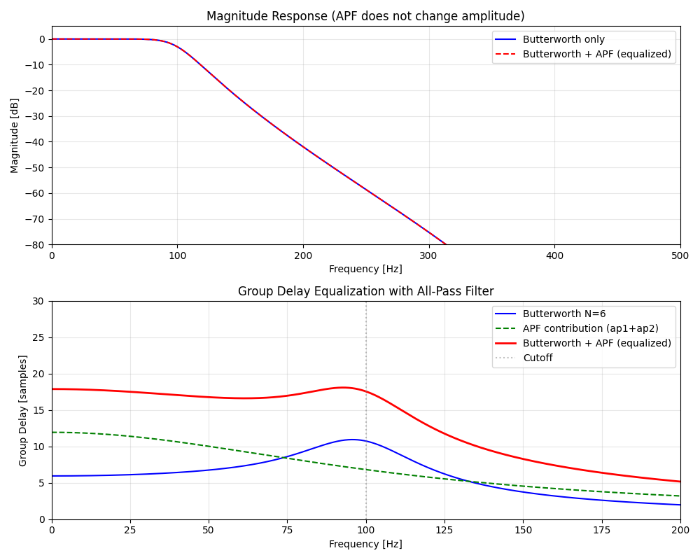
The top panel shows the Butterworth-only and equalized magnitude responses overlapping exactly, with a measured maximum difference of 0.000000 dB (below floating-point resolution). The bottom panel shows the passband (0-100 Hz) group delay spread shrinking from 4.994 samples (Butterworth alone) to 1.473 samples after adding the all-pass sections — roughly a 3.4x reduction — confirming that group delay can be substantially flattened without altering the amplitude response at all.
Caveat: the placement of the all-pass group-delay peaks is a critical design choice, not an afterthought. Placing the peaks near the cutoff instead (where the Butterworth filter’s own delay is already highest) makes the spread worse, not better — empirically, the spread grows from 4.994 to 7.041 samples with that placement. Flattening requires boosting the region where the target filter’s delay is low, not adding more delay where it is already high; simply cascading all-pass sections does not automatically equalize the response. In practice, the pole radius and angle of each all-pass section are typically optimized (e.g., by least-squares minimization of the group delay error) rather than chosen by hand.
IIR Filter Group Delay Comparison
fs = 1000
fc = 100
N = 6

filters = {
    'Butterworth': butter(N, fc, fs=fs, output='ba'),
    'Chebyshev I (1 dB)': cheby1(N, 1, fc, fs=fs, output='ba'),
    'Elliptic (1 dB, 60 dB)': ellip(N, 1, 60, fc, fs=fs, output='ba'),
    'Bessel': bessel(N, fc, norm='mag', fs=fs, output='ba'),
}

fig, axes = plt.subplots(2, 1, figsize=(10, 8))

gd_stats = {}
for name, (b, a) in filters.items():
    w_hz, H = freqz(b, a, worN=4096, fs=fs)
    w_gd, gd = group_delay((b, a), w=4096, fs=fs)
    axes[0].plot(w_hz, 20 * np.log10(np.abs(H) + 1e-12), label=name)
    axes[1].plot(w_gd, gd, label=name)

    mask_pb = (w_gd >= 0) & (w_gd <= fc)
    gd_stats[name] = (gd[mask_pb].min(), gd[mask_pb].max(), gd[mask_pb].std())

axes[0].set_xlabel('Frequency [Hz]')
axes[0].set_ylabel('Magnitude [dB]')
axes[0].set_title(f'Magnitude Response: IIR Filter Comparison (N={N}, fc={fc} Hz)')
axes[0].set_xlim(0, 300)
axes[0].set_ylim(-80, 5)
axes[0].axvline(fc, color='gray', linestyle=':', alpha=0.5)
axes[0].legend()
axes[0].grid(True, alpha=0.3)

axes[1].set_xlabel('Frequency [Hz]')
axes[1].set_ylabel('Group Delay [samples]')
axes[1].set_title('Group Delay: IIR Filter Comparison')
axes[1].set_xlim(0, 300)
axes[1].set_ylim(0, 50)
axes[1].axvline(fc, color='gray', linestyle=':', alpha=0.5)
axes[1].legend()
axes[1].grid(True, alpha=0.3)

plt.tight_layout()
plt.savefig('iir_filter_comparison.png')

print("Passband (0-100 Hz) group delay stats (min, max, std) [samples]:")
for name, (mn, mx, sd) in gd_stats.items():
    print(f"  {name}: min={mn:.3f}, max={mx:.3f}, std={sd:.3f}")
Output:
Passband (0-100 Hz) group delay stats (min, max, std) [samples]:
  Butterworth: min=5.946, max=10.940, std=1.676
  Chebyshev I (1 dB): min=6.858, max=31.263, std=4.781
  Elliptic (1 dB, 60 dB): min=5.412, max=46.929, std=7.203
  Bessel: min=4.160, max=4.596, std=0.129
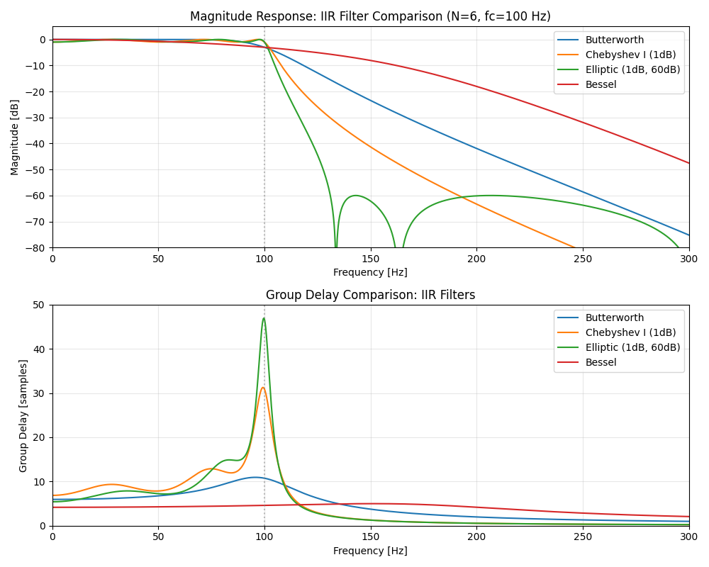
Comparing the passband (0-100 Hz) group delay standard deviation, the Bessel filter is by far the flattest at 0.129 samples (ranging only 4.160-4.596 samples), numerically confirming its Maximally Flat Group Delay design objective. The elliptic filter, at the other extreme, has a standard deviation of 7.203 samples (ranging 5.412-46.929 samples) — the largest group delay peak of the four, reflecting the trade-off against its minimum-order, sharpest-transition design. Chebyshev Type I sits in between at 4.781 samples, confirming with real numbers the qualitative ordering summarized in the group delay comparison table above.
Summary
| Concept | Definition / Property | Practical significance |
|---|---|---|
| Phase spectrum | \(\phi(\omega) = \angle H(e^{j\omega})\) ; requires unwrapping for continuity | Determines how each frequency component is time-shifted |
| Group delay | \(\tau_g(\omega) = -d\phi/d\omega\) ; units: samples | Quantifies frequency-dependent signal packet delay |
| Linear phase | \(\phi(\omega) = -\omega\tau_0\) ; constant group delay \(\tau_0\) | Output is a pure time-shifted copy of the input |
| FIR linear phase | Symmetric coefficients \(h[n]=h[N-1-n]\) ; \(\tau_g = (N-1)/2\) samples | Exact linear phase guaranteed; magnitude and phase independently designable |
| IIR nonlinear phase | Fundamental property of stable IIR filters with poles inside the unit circle | Trade-off against amplitude sharpness is unavoidable |
| All-pass filter | \(\lvert H_{AP} \rvert = 1\) for all \(\omega\) ; phase freely controllable | Phase equalization without changing amplitude |
| Phase equalization | Cascade IIR + all-pass; optimize for flat total group delay | Reduces waveform distortion in real-time IIR systems |
Practical Filter Selection Guide
| Requirement | Recommended approach |
|---|---|
| Waveform shape preservation is critical (ECG, impulse response) | Linear-phase FIR filter (firwin) |
| Sharp magnitude cutoff, phase distortion acceptable | Elliptic IIR filter (ellip) |
| Flat group delay in passband with IIR | Bessel filter (bessel) |
| IIR filter with phase distortion reduction | IIR + all-pass equalization |
| Offline processing, zero phase shift required | filtfilt / sosfiltfilt (forward-backward filtering) |
| Real-time processing with minimum total delay | Low-order IIR (Butterworth) + group delay monitoring |
Related Articles
- Fast Fourier Transform (FFT): Theory and Python Implementation - The foundation of phase spectrum analysis.
- FIR and IIR Filter Comparison - Foundational comparison of FIR and IIR filter properties.
- Butterworth Filter Design: Theory and Python Implementation - Canonical example of IIR nonlinear phase behavior.
- Chebyshev Filter Design and Python Implementation - Sharper transition at the cost of greater group delay distortion.
- Elliptic Filter Design and Python Implementation - Minimum-order design with maximum group delay distortion.
- Bessel Filter Design and Python Implementation - Maximum-flat group delay IIR filter.
- Short-Time Fourier Transform (STFT): Theory and Python Implementation - Time-frequency analysis that captures phase evolution over time.
- Hilbert Transform and Instantaneous Frequency Analysis - Instantaneous phase and frequency, closely related to group delay concepts.
References
- Oppenheim, A. V., & Schafer, R. W. (2009). Discrete-Time Signal Processing (3rd ed.). Prentice Hall.
- Proakis, J. G., & Manolakis, D. G. (2006). Digital Signal Processing: Principles, Algorithms, and Applications (4th ed.). Pearson.
- Zölzer, U. (2011). DAFX: Digital Audio Effects (2nd ed.). Wiley.
- Smith, J. O. (2007). Introduction to Digital Filters with Audio Applications. W3K Publishing. https://ccrma.stanford.edu/~jos/filters/
- Zhang, et al. (2025). A group delay equalization method for filters based on DGS NGD structure. Electromagnetics. https://doi.org/10.1080/02726343.2025.2548618
- SciPy
scipy.signal.group_delaydocumentation - SciPy
scipy.signal.freqzdocumentation