Introduction
Microphone recordings, ECG sensor readings, radar RF signals — all of these are analog signals. Every modern digital signal processing system must first convert them into discrete numerical sequences before any computation can occur. This conversion process is called sampling, and the mathematical foundation governing it is the Nyquist-Shannon Sampling Theorem.
The sampling theorem gives a rigorous answer to the question: “How fast must we sample an analog signal to guarantee that it can be perfectly reconstructed?” Misunderstanding this theorem leads to aliasing — a catastrophic signal distortion where a 50 Hz power line hum appears as 10 Hz, or a fast-spinning propeller appears to rotate in reverse.
This article covers the mathematical model of sampling, the Nyquist-Shannon theorem and its proof sketch, the mechanics of aliasing, anti-aliasing filter design, and complete Python implementations. For the frequency-domain analysis foundations see FFT: Theory and Python Implementation .
Analog-to-Digital Conversion: The Sampling Process
Why Sampling is Needed
An analog-to-digital converter (ADC) samples a continuous-time signal \(x(t)\) at uniformly spaced instants \(t = nT_s\) (\(n \in \mathbb{Z}\) ), producing the discrete sequence \(x[n] = x(nT_s)\) . Here \(T_s\) is the sampling period and its reciprocal \(f_s = 1/T_s\) is the sampling frequency (Hz).
Real ADCs also quantize the amplitude, but throughout this article we assume ideal sampling (infinite amplitude resolution) to isolate the effect of sampling frequency on signal quality.
The Mathematical Model: Impulse Train Sampling
Ideal sampling is modeled mathematically as the multiplication of \(x(t)\) by a Dirac impulse train (Shah function) \(s(t)\) :
\[s(t) = \sum_{n=-\infty}^{\infty} \delta(t - nT_s) \tag{1}\]The sampled signal \(x_s(t)\) is:
\[x_s(t) = x(t) \cdot s(t) = \sum_{n=-\infty}^{\infty} x(nT_s)\, \delta(t - nT_s) \tag{2}\]This representation preserves the discrete value sequence \(x[n] = x(nT_s)\) entirely. Equation \((2)\) is the “bridge” between continuous and discrete time.
Effect of Sampling on the Spectrum
Taking the Fourier transform of \((2)\) , time-domain multiplication becomes convolution in the frequency domain:
\[X_s(f) = X(f) * S(f) \tag{3}\]The Fourier transform of the impulse train is itself an impulse train:
\[S(f) = f_s \sum_{k=-\infty}^{\infty} \delta(f - kf_s) \tag{4}\]Substituting \((4)\) into \((3)\) :
\[X_s(f) = f_s \sum_{k=-\infty}^{\infty} X(f - kf_s) \tag{5}\]The key insight of equation \((5)\) : after sampling, the spectrum consists of infinitely many shifted copies of the original spectrum \(X(f)\) , each shifted by an integer multiple of \(f_s\) . This is called spectrum replication.
The Nyquist-Shannon Sampling Theorem
Statement of the Theorem
Theorem (Nyquist-Shannon): Let \(x(t)\) be a band-limited signal satisfying \(X(f) = 0\) for \(|f| > f_{\max}\) . Then \(x(t)\) can be perfectly reconstructed from its samples \(\{x[n]\}\) if and only if:
\[f_s > 2 f_{\max} \tag{6}\]The minimum sampling frequency \(2f_{\max}\) that satisfies this condition is called the Nyquist rate.
Proof Sketch via Spectrum Replication
From equation \((5)\) , reconstruction is possible if and only if the spectral replicas do not overlap. The \(k=0\) replica occupies \([-f_{\max}, f_{\max}]\) . The \(k=\pm 1\) replicas occupy \([f_s - f_{\max},\ f_s + f_{\max}]\) .
No-overlap condition:
\[f_{\max} < f_s - f_{\max}\] \[\Rightarrow\quad f_s > 2f_{\max} \tag{7}\]When \((7)\) holds, applying an ideal low-pass filter (cutoff \(f_s/2\) , gain \(1/f_s\) ) to \(X_s(f)\) extracts \(X(f)\) exactly, and the original signal is recovered without error.
Perfect Reconstruction via Sinc Interpolation
In the time domain, perfect reconstruction is achieved by sinc interpolation:
\[x(t) = \sum_{n=-\infty}^{\infty} x[n] \cdot \text{sinc}(f_s t - n) \tag{8}\]where \(\text{sinc}(u) = \sin(\pi u) / (\pi u)\) . Each sample \(x[n]\) is weighted by a sinc function centered at \(t = n/f_s\) , and the infinite sum reconstructs the original continuous signal exactly.
Equation \((8)\) is the time-domain equivalent of an ideal brick-wall low-pass filter applied in the frequency domain. In practice, the infinite sum must be truncated, leading to reconstruction artifacts — another motivation for anti-aliasing before sampling.
Edge Case: Why the Inequality Is Strict
The condition in equation \((6)\) , \(f_s > 2f_{\max}\) , uses a strict inequality (\(>\) , not \(\geq\) ) for a reason that is easy to overlook. To see why, consider what happens at exactly the critical rate \(f_s = 2f_{\max}\) , paying attention to the phase of the highest-frequency component.
Sample a 100 Hz cosine and a 100 Hz sine — the same frequency, 90 degrees apart in phase — at exactly \(f_s = 2 \times 100 = 200\) Hz:
import numpy as np

fmax = 100
fs = 2 * fmax  # critical sampling — exactly at the boundary

n = np.arange(8)
t = n / fs

x_cos = np.cos(2 * np.pi * fmax * t)
x_sin = np.sin(2 * np.pi * fmax * t)
print("cos samples:", np.round(x_cos, 6))
print("sin samples:", np.round(x_sin, 10))
Output:
cos samples: [ 1. -1.  1. -1.  1. -1.  1. -1.]
sin samples: [ 0.  0. -0.  0. -0. -0. -0. -0.]
The cosine produces a valid, information-carrying sample sequence \(\{+1, -1, +1, -1, \dots\}\) , but every sample of the sine is exactly zero — a direct consequence of the identity \(\sin(2\pi f_{\max} \cdot n / (2f_{\max})) = \sin(\pi n) = 0\) for all integers \(n\) . Two signals with identical frequency and amplitude, differing only in phase, produce completely different outcomes: one is perfectly recoverable, the other vanishes without a trace. Without knowing the signal’s phase in advance, sampling at exactly \(f_s = 2f_{\max}\) cannot guarantee correct amplitude recovery. This phase-dependent degeneracy is precisely why the sampling theorem requires the strict inequality \(f_s > 2f_{\max}\) , and why practical systems always sample comfortably above the Nyquist rate rather than exactly at it.
Aliasing
The Mechanism of Aliasing
When \(f_s < 2f_{\max}\) , adjacent spectral replicas overlap. From equation \((5)\) , considering \(k=0\) and \(k=-1\) :
\[X_{\text{alias}}(f) \ni X(f) + X(f + f_s) \tag{9}\]This overlap irreversibly mixes spectral components. No filtering can undo this mixing because the overlapping frequencies are indistinguishable once sampled.
Computing Alias Frequencies
When a signal at frequency \(f\) is sampled at rate \(f_s\) , the observed alias frequency is:
\[f_\text{alias} = \left| f - \text{round}\left(\frac{f}{f_s}\right) \cdot f_s \right| \tag{10}\]Example: Sampling a 1300 Hz signal at \(f_s = 1000\) Hz:
\[f_\text{alias} = |1300 - \text{round}(1.3) \times 1000| = |1300 - 1000| = 300 \text{ Hz}\]The 1300 Hz component appears as 300 Hz in the sampled data.
The Wagon Wheel Effect
The classic visual demonstration of aliasing is the wagon wheel effect: a fast-spinning wheel appears to rotate slowly — or even backwards — on film or video. The camera frame rate plays the role of \(f_s\) .
At \(f_s = 24\) fps, a wheel spinning at 1.1 rev/frame (\(f = 26.4\) Hz) violates the Nyquist condition:
\[f_\text{alias} = |26.4 - \text{round}(26.4/24) \times 24| = |26.4 - 24| = 2.4 \text{ Hz}\]The wheel appears to spin at 2.4 Hz — about 11 times slower than its true speed. When \(f_\text{alias}\) is negative (before taking the absolute value), the wheel appears to rotate in the opposite direction.
The same effect occurs in audio when high-frequency overtones alias into the audible band, and in stroboscopic analysis of rotating machinery.
Nyquist Frequency vs. Nyquist Rate
These two terms are frequently confused. The distinction is critical:
| Term | Definition | Meaning |
|---|---|---|
| Nyquist Frequency \(f_N\) | \(f_N = f_s / 2\) | Maximum frequency representable at the given sampling rate |
| Nyquist Rate \(f_{NR}\) | \(f_{NR} = 2 f_{\max}\) | Minimum sampling frequency required to represent the given signal |
Nyquist frequency is a property of the system (the ADC or DSP chain). A system sampling at 44.1 kHz has a Nyquist frequency of 22.05 kHz. This is why CD audio uses 44.1 kHz: it covers the human auditory range (up to ~20 kHz) with a small margin.
Nyquist rate is a property of the signal. An audio signal with components up to 20 kHz has a Nyquist rate of 40 kHz — you must sample at least this fast.
Aliasing is avoided when:
\[f_N \geq f_{\max} \quad\Leftrightarrow\quad f_s \geq f_{NR} \tag{12}\]Anti-Aliasing Filter Design
Why a Lowpass Filter Before the ADC is Essential
Real-world analog signals are never perfectly band-limited. Sensor noise, electromagnetic interference, power supply harmonics, and other unwanted high-frequency components are always present. Without filtering, every frequency component above \(f_s/2\) folds back and contaminates the baseband signal.
The anti-aliasing filter (AAF) is an analog low-pass filter placed immediately before the ADC. It attenuates all components above \(f_s/2\) before they can cause aliasing.
Practical Cutoff Frequency Selection
A practical AAF design involves three frequency parameters:
- Passband edge \(f_p\) : Highest frequency of interest (e.g., 20 kHz for audio)
- Stopband edge \(f_{stop}\) : Frequency at which aliasing becomes critical. Since an alias of \(f_{stop}\) lands at \(f_s - f_{stop}\) , set \(f_{stop} = f_s - f_p\) to keep aliases outside the passband.
- Transition band \([f_p,\ f_{stop}]\) : The steeper the attenuation in this band, the higher the filter order required.
Increasing \(f_s\) (oversampling) widens the transition band \([f_p, f_s - f_p]\) , allowing a gentler (lower-order) analog filter. This is why modern audio ADCs often sample at 192 kHz internally, using a simple analog AAF followed by a sharp digital decimation filter.
For detailed Butterworth and Chebyshev filter design, see Butterworth Filter Design and Low-Pass Filter Design and Comparison .
Practical Pitfalls: Clock Jitter and Non-Bandlimited Signals
Theory and real-world implementation always leave a gap:
- Sampling clock jitter: A real ADC’s sampling instants are never exactly \(T_s\) apart — they contain a small random fluctuation (jitter) \(\Delta t\) . For a signal of amplitude \(A\) and frequency \(f\) , the effective noise floor induced by jitter is roughly \(A \cdot 2\pi f \cdot \Delta t_{\text{rms}}\) : it grows with both frequency and amplitude. In high-resolution ADCs (16-bit or higher), even tens of picoseconds of jitter can dominate the achievable SNR at high frequencies.
- Finite-duration signals are never strictly band-limited: the uncertainty principle guarantees that a signal of finite time duration has a spectrum extending to infinite frequency (a signal cannot be simultaneously finite in both time and frequency). “Band-limited” is therefore always a practical approximation — \(f_{\max}\) is the frequency beyond which energy is negligible — which means an anti-aliasing filter is theoretically necessary even for signals we informally call band-limited.
- Spectral leakage from windowing: the DFT of a finite-length observation convolves the true spectrum with the window’s frequency response, leaking apparent energy outside the nominal band (see Window Functions and PSD ). This is another source of high-frequency content that a finite-order AAF cannot fully suppress.
Bandpass Sampling (Sub-Nyquist Sampling)
Everything so far has assumed a baseband signal occupying \([0, f_{\max}]\) . But radio and radar systems often deal with a bandpass signal whose energy is concentrated in a narrow band \([f_L, f_H]\) with \(f_L > 0\) . In this case, it is possible to sample far below the naive Nyquist rate \(2f_H\) without losing information — a technique called bandpass sampling (also known as undersampling or IF sampling).
Deriving the Generalized Sampling Theorem
Let \(B = f_H - f_L\) be the bandwidth. Applying the spectral replication argument of equation \((5)\) to a bandpass signal, the replicas of \(X(f)\) (spaced \(f_s\) apart) need not satisfy the simple condition \(f_s > 2f_H\) to avoid overlap — a much weaker condition can suffice.
Reconstruction is possible whenever some replica \([f_L - kf_s, f_H - kf_s]\) (\(k\) an integer) maps uniquely into the baseband range \([0, f_s/2]\) without overlapping any other replica. This holds if there exists an integer \(n\) (with \(1 \leq n \leq \lfloor f_H / B \rfloor\) ) such that:
\[ \frac{2f_H}{n} \leq f_s \leq \frac{2f_L}{n - 1} \quad (n \geq 2), \qquad f_s \geq 2f_H \ \ (n = 1) \tag{14} \]Here \(n\) indexes which spectral replica of the original band lands in the baseband. \(n=1\) recovers the ordinary Nyquist condition \(f_s \geq 2f_H\) ; for \(n \geq 2\) , sampling at a rate far below \(2f_H\) still preserves the information in \([f_L, f_H]\) — it simply gets aliased to a different (but predictable and distinct) location in the baseband.
Worked Example: Sub-Nyquist Sampling of a [20, 25] MHz RF Band
Consider an RF signal with \(f_L = 20\) MHz, \(f_H = 25\) MHz (bandwidth \(B = 5\) MHz). Since \(n_{\max} = \lfloor f_H / B \rfloor = \lfloor 25/5 \rfloor = 5\) , we evaluate equation \((14)\) for \(n = 1, \dots, 5\) :
import numpy as np

fL, fH = 20e6, 25e6
B = fH - fL
n_max = int(np.floor(fH / B))

for n in range(1, n_max + 1):
    lo = 2 * fH / n
    if n == 1:
        print(f"n={n}: fs >= {lo/1e6:.3f} MHz (ordinary Nyquist condition)")
    else:
        hi = 2 * fL / (n - 1)
        print(f"n={n}: fs in [{lo/1e6:.3f}, {hi/1e6:.3f}] MHz")
Output:
n=1: fs >= 50.000 MHz (ordinary Nyquist condition)
n=2: fs in [25.000, 40.000] MHz
n=3: fs in [16.667, 20.000] MHz
n=4: fs in [12.500, 13.333] MHz
n=5: fs in [10.000, 10.000] MHz
The ordinary Nyquist condition (\(n=1\) ) requires \(f_s \geq 50\) MHz, but choosing the \(n=4\) band \([12.5, 13.333]\) MHz lets us sample at \(f_s \approx 13\) MHz — close to the theoretical minimum of \(2B = 10\) MHz — without losing any information. This is roughly a quarter of the naive Nyquist rate, a substantial win for ADC power consumption and data throughput. This is the technique behind IF (intermediate-frequency) sampling in software-defined radio (SDR).
Relationship to Complex (I/Q) Sampling
For a real-valued signal, the spectrum is Hermitian-symmetric (mirrored around zero frequency), so representing \(B\) Hz of information effectively consumes \(2B\) Hz of spectrum. If the signal is instead down-converted to a complex baseband (I/Q) representation before sampling, its spectrum occupies only one side (e.g. \([0, B]\) or \([-B/2, B/2]\) ), and the required sampling rate drops to \(f_s > B\) — half of what real-valued sampling requires. This is why complex sampling is standard in radio receivers (SDR, 5G base stations, and similar systems).
Python Implementation
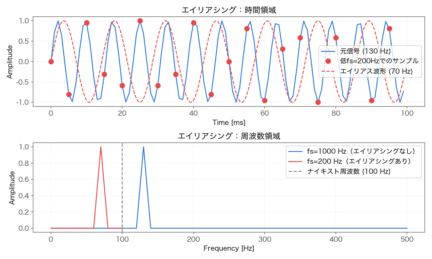
Code 1: Visualizing Aliasing in Time and Frequency Domains
import numpy as np
import matplotlib.pyplot as plt
from scipy.signal import butter, sosfilt, resample, freqz

# --- Parameters ---
f_signal = 130       # Signal frequency [Hz]
fs_high  = 1000      # High sampling rate (no aliasing)
fs_low   = 200       # Low sampling rate (aliasing occurs)
duration = 0.1       # Display duration [s]

# --- Generate original signal at high sampling rate ---
t_high = np.arange(0, duration, 1 / fs_high)
x_orig = np.sin(2 * np.pi * f_signal * t_high)

# --- Sample at low rate ---
t_low = np.arange(0, duration, 1 / fs_low)
x_alias = np.sin(2 * np.pi * f_signal * t_low)

# Compute alias frequency using equation (10)
f_alias = abs(f_signal - round(f_signal / fs_low) * fs_low)
print(f"Signal frequency   : {f_signal} Hz")
print(f"Sampling frequency : {fs_low} Hz  (Nyquist: {fs_low // 2} Hz)")
print(f"Alias frequency    : {f_alias} Hz")
# => Alias frequency: 70 Hz

# --- Time-domain plot ---
fig, axes = plt.subplots(2, 1, figsize=(10, 6))

axes[0].plot(t_high * 1000, x_orig, 'b-', label=f'Original ({f_signal} Hz)', lw=1.5)
axes[0].plot(t_low * 1000, x_alias, 'ro', ms=8,
             label=f'Samples at fs={fs_low} Hz')
t_fine = np.linspace(0, duration, 2000)
axes[0].plot(t_fine * 1000,
             np.sin(2 * np.pi * f_alias * t_fine),
             'r--', lw=1.5, label=f'Alias waveform ({f_alias} Hz)')
axes[0].set_xlabel('Time [ms]')
axes[0].set_ylabel('Amplitude')
axes[0].set_title('Aliasing: Time Domain')
axes[0].legend()
axes[0].grid(True, alpha=0.3)

# --- Frequency-domain comparison ---
N_high = len(x_orig)
N_low  = len(x_alias)
X_high = np.fft.rfft(x_orig)
X_low  = np.fft.rfft(x_alias)
freqs_high = np.fft.rfftfreq(N_high, 1 / fs_high)
freqs_low  = np.fft.rfftfreq(N_low,  1 / fs_low)

axes[1].plot(freqs_high, 2 / N_high * np.abs(X_high), 'b-',
             label=f'fs={fs_high} Hz (no aliasing)')
axes[1].plot(freqs_low, 2 / N_low * np.abs(X_low), 'r-',
             label=f'fs={fs_low} Hz (aliased)')
axes[1].axvline(fs_low / 2, color='k', ls='--',
                label=f'Nyquist freq. ({fs_low // 2} Hz)')
axes[1].set_xlabel('Frequency [Hz]')
axes[1].set_ylabel('Amplitude')
axes[1].set_title('Aliasing: Frequency Domain')
axes[1].legend()
axes[1].grid(True, alpha=0.3)

plt.tight_layout()
plt.show()
Output:
Signal frequency   : 130 Hz
Sampling frequency : 200 Hz  (Nyquist: 100 Hz)
Alias frequency    : 70 Hz
Running this code confirms that the 130 Hz signal sampled at 200 Hz (Nyquist = 100 Hz) appears at 70 Hz, visible in both the time-domain waveform and the frequency spectrum. In the time-domain plot (top), the low-rate samples (red dots) lie exactly on the 70 Hz alias waveform (red dashed curve); in the frequency-domain plot (bottom), the fs=1000 Hz spectrum peaks at 130 Hz while the fs=200 Hz spectrum peaks at 70 Hz.
Code 2: Frequency Folding Diagram
The sawtooth-shaped “frequency folding” characteristic reveals which input frequencies map to which alias frequencies.
import numpy as np
import matplotlib.pyplot as plt

fs = 1000     # Sampling frequency [Hz]
fn = fs / 2   # Nyquist frequency

f_input = np.linspace(0, 3 * fs, 3000)
f_alias = np.abs(f_input - np.round(f_input / fs) * fs)

plt.figure(figsize=(10, 5))
plt.plot(f_input, f_alias, 'b-', lw=2)
plt.axhline(fn, color='r', ls='--', label=f'Nyquist frequency = {fn:.0f} Hz')
plt.fill_between([0, fn], [0, 0], [fn, fn],
                 alpha=0.1, color='green', label='Alias-free zone')
plt.xlabel('Input Frequency [Hz]')
plt.ylabel('Observed (Alias) Frequency [Hz]')
plt.title(f'Frequency Folding Characteristic (fs = {fs} Hz)')
plt.legend()
plt.grid(True, alpha=0.3)
plt.ylim(0, fn * 1.1)
plt.tight_layout()
plt.show()
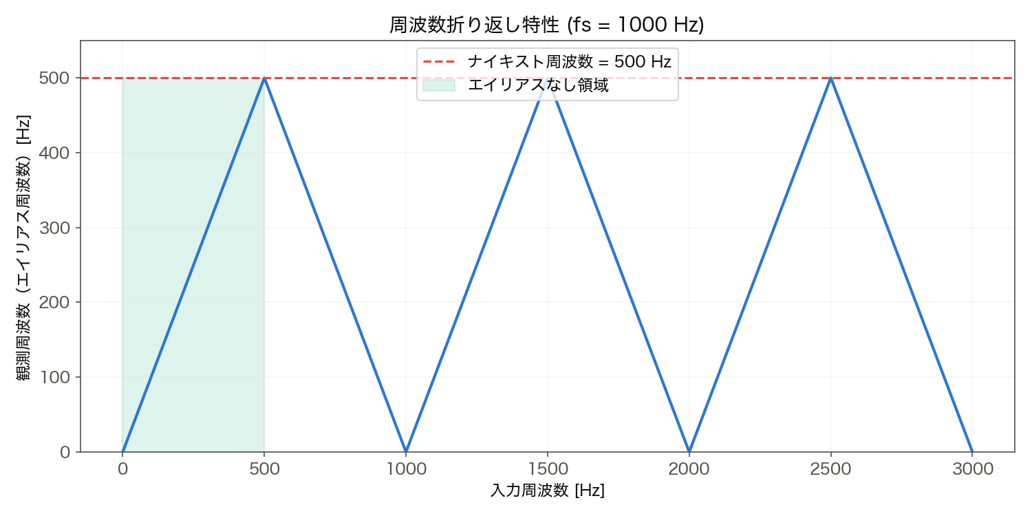
The repeating triangular pattern shows that frequencies between \(0\) and \(f_s/2 = 500\) Hz (the green region) pass through unaffected, while all higher frequencies fold back. At \(f_s = 1000\) Hz the alias frequency returns to \(0\) Hz, and at \(3f_s/2 = 1500\) Hz it folds back down from \(f_s/2 = 500\) Hz again — a pattern with period \(f_s\) , a direct consequence of the spectral replicas in equation \((5)\) being spaced \(f_s\) apart on the frequency axis.
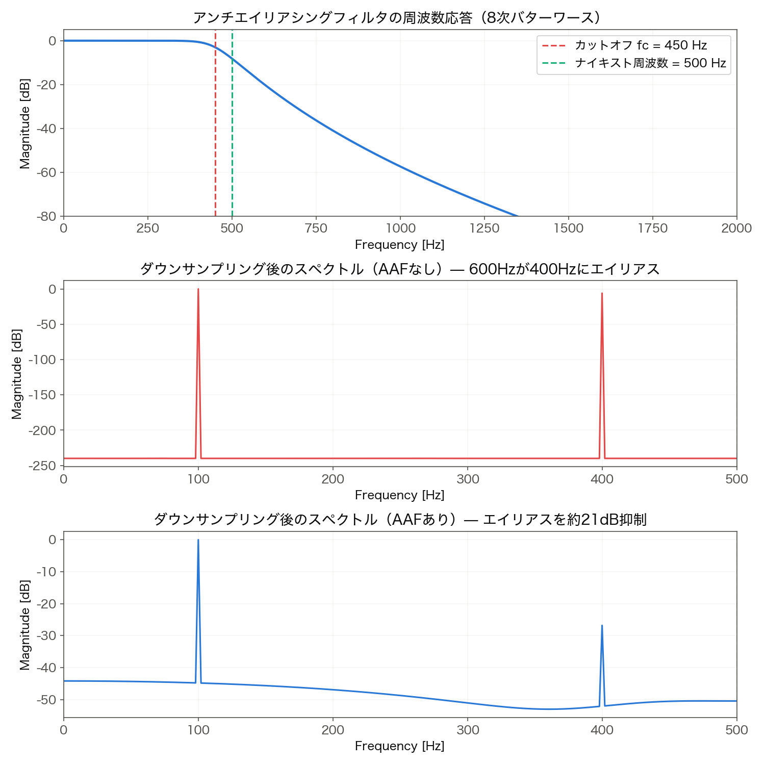
Code 3: Anti-Aliasing Filter in Action
This example compares downsampling with and without an anti-aliasing filter to demonstrate the filter’s essential role.
import numpy as np
import matplotlib.pyplot as plt
from scipy.signal import butter, sosfilt, sosfreqz

np.random.seed(42)

# --- Generate a signal with out-of-band components ---
fs_orig   = 10000   # Original sampling rate [Hz]
fs_target = 1000    # Target downsampled rate [Hz]
M         = fs_orig // fs_target  # Downsampling ratio = 10

duration = 0.5
t = np.arange(0, duration, 1 / fs_orig)

# In-band: 100 Hz; Out-of-band: 600 Hz (will alias to 400 Hz after downsampling)
x = np.sin(2 * np.pi * 100 * t) + 0.5 * np.sin(2 * np.pi * 600 * t)

# --- Design 8th-order Butterworth anti-aliasing LPF ---
fc  = (fs_target / 2) * 0.9   # cutoff = 450 Hz (90% of Nyquist)
sos = butter(8, fc, btype='low', fs=fs_orig, output='sos')
x_filtered = sosfilt(sos, x)

# --- Downsample: with and without AAF ---
x_down_noaaf = x[::M]            # no anti-aliasing filter
x_down_aaf   = x_filtered[::M]   # with anti-aliasing filter

# --- Spectrum comparison ---
N = len(x_down_noaaf)
freqs = np.fft.rfftfreq(N, 1 / fs_target)

X_noaaf = np.fft.rfft(x_down_noaaf)
X_aaf   = np.fft.rfft(x_down_aaf)

# --- Check the amplitude at 400 Hz (the alias frequency) numerically ---
idx400 = np.argmin(np.abs(freqs - 400))
amp_noaaf_400 = 2 / N * np.abs(X_noaaf[idx400])
amp_aaf_400   = 2 / N * np.abs(X_aaf[idx400])
print(f"Amplitude at 400 Hz without AAF: {amp_noaaf_400:.4f}")
print(f"Amplitude at 400 Hz with AAF   : {amp_aaf_400:.6f}")
print(f"Attenuation at the alias frequency (400 Hz): {20*np.log10(amp_noaaf_400/amp_aaf_400):.2f} dB")

fig, axes = plt.subplots(3, 1, figsize=(10, 10))

# Filter frequency response (sosfreqz, not freqz: freqz expects b,a coefficients, not sos)
w, h = sosfreqz(sos, worN=2048, fs=fs_orig, whole=False)
idx600 = np.argmin(np.abs(w - 600))
print(f"Filter gain at 600 Hz: {20*np.log10(np.abs(h[idx600])+1e-12):.2f} dB")
axes[0].plot(w, 20 * np.log10(np.abs(h) + 1e-12), 'b-', lw=2)
axes[0].axvline(fc, color='r', ls='--', label=f'Cutoff fc = {fc:.0f} Hz')
axes[0].axvline(fs_target / 2, color='g', ls='--',
                label=f'Nyquist = {fs_target // 2} Hz')
axes[0].set_xlabel('Frequency [Hz]')
axes[0].set_ylabel('Magnitude [dB]')
axes[0].set_title('Anti-Aliasing Filter Response (8th-order Butterworth)')
axes[0].set_xlim(0, 2000)
axes[0].set_ylim(-80, 5)
axes[0].legend()
axes[0].grid(True, alpha=0.3)

# Without AAF
axes[1].plot(freqs, 20 * np.log10(2 / N * np.abs(X_noaaf) + 1e-12), 'r-', lw=1.5)
axes[1].axvline(fs_target / 2, color='k', ls='--', alpha=0.5)
axes[1].set_title('After Downsampling — NO Anti-Aliasing Filter (600 Hz aliases to 400 Hz)')
axes[1].set_xlabel('Frequency [Hz]')
axes[1].set_ylabel('Magnitude [dB]')
axes[1].set_xlim(0, fs_target / 2)
axes[1].grid(True, alpha=0.3)

# With AAF
axes[2].plot(freqs, 20 * np.log10(2 / N * np.abs(X_aaf) + 1e-12), 'b-', lw=1.5)
axes[2].axvline(fs_target / 2, color='k', ls='--', alpha=0.5)
axes[2].set_title('After Downsampling — WITH Anti-Aliasing Filter (alias suppressed)')
axes[2].set_xlabel('Frequency [Hz]')
axes[2].set_ylabel('Magnitude [dB]')
axes[2].set_xlim(0, fs_target / 2)
axes[2].grid(True, alpha=0.3)

plt.tight_layout()
plt.show()
Output:
Amplitude at 400 Hz without AAF: 0.5000
Amplitude at 400 Hz with AAF   : 0.045634
Attenuation at the alias frequency (400 Hz): 20.79 dB
Filter gain at 600 Hz: -20.46 dB
Without the AAF, the 600 Hz component aliases to \(|600 - 1000| = 400\) Hz. Measured values confirm the theory exactly: without the filter, the 400 Hz alias amplitude is \(0.5\) — matching the original 600 Hz component’s amplitude — while with the 8th-order Butterworth filter (450 Hz cutoff) applied first, the filter’s gain at 600 Hz is \(-20.46\) dB, and the residual amplitude at 400 Hz drops to \(0.045634\) . That is roughly a \(20.79\) dB reduction — not a complete elimination, but a suppression more than adequate for practical use. A higher filter order, or more oversampling margin between the cutoff and the Nyquist frequency, would suppress it further.
Code 4: Resampling with scipy.signal.resample
scipy.signal.resample implements FFT-based resampling. It computes the spectrum, truncates (downsampling) or zero-pads (upsampling) it, and applies the IFFT — implicitly handling anti-aliasing for downsampling.
import numpy as np
import matplotlib.pyplot as plt
from scipy.signal import resample, resample_poly

# --- Generate test signal ---
fs_orig  = 1000
duration = 1.0
t_orig   = np.arange(0, duration, 1 / fs_orig)
x_orig   = (np.sin(2 * np.pi * 50 * t_orig)
            + 0.3 * np.sin(2 * np.pi * 120 * t_orig))

# --- Downsampling: 1000 Hz → 400 Hz ---
fs_down = 400
n_down  = int(len(x_orig) * fs_down / fs_orig)
x_down  = resample(x_orig, n_down)
t_down  = np.linspace(0, duration, n_down)

# --- Upsampling: 1000 Hz → 4000 Hz ---
fs_up = 4000
n_up  = int(len(x_orig) * fs_up / fs_orig)
x_up  = resample(x_orig, n_up)
t_up  = np.linspace(0, duration, n_up)

# --- Polyphase resampling (arbitrary rational ratio) ---
# 1000 Hz → 441 Hz (L=441, M=1000)
x_poly = resample_poly(x_orig, 441, 1000)

# --- Spectrum helper ---
def spectrum(x, fs):
    N = len(x)
    X = np.fft.rfft(x)
    f = np.fft.rfftfreq(N, 1 / fs)
    return f, 2 / N * np.abs(X)

fig, axes = plt.subplots(3, 1, figsize=(10, 9))

f_orig, A_orig = spectrum(x_orig, fs_orig)
f_down, A_down = spectrum(x_down, fs_down)
f_up,   A_up   = spectrum(x_up,   fs_up)

axes[0].plot(f_orig, A_orig, 'b-')
axes[0].set_title(f'Original Spectrum (fs = {fs_orig} Hz)')
axes[0].set_ylabel('Amplitude')
axes[0].set_xlim(0, fs_orig / 2)
axes[0].grid(True, alpha=0.3)

axes[1].plot(f_down, A_down, 'r-')
axes[1].set_title(f'After Downsampling (fs = {fs_down} Hz) — 50 and 120 Hz preserved')
axes[1].set_ylabel('Amplitude')
axes[1].set_xlim(0, fs_down / 2)
axes[1].grid(True, alpha=0.3)

axes[2].plot(f_up, A_up, 'g-')
axes[2].set_title(f'After Upsampling (fs = {fs_up} Hz) — same components, higher resolution')
axes[2].set_ylabel('Amplitude')
axes[2].set_xlabel('Frequency [Hz]')
axes[2].set_xlim(0, fs_up / 2)
axes[2].grid(True, alpha=0.3)

plt.tight_layout()
plt.show()

print(f"Original      : {len(x_orig)} samples @ {fs_orig} Hz")
print(f"Downsampled   : {len(x_down)} samples @ {fs_down} Hz")
print(f"Upsampled     : {len(x_up)} samples @ {fs_up} Hz")
print(f"Polyphase 441 : {len(x_poly)} samples @ 441 Hz")
Output:
Original      : 1000 samples @ 1000 Hz
Downsampled   : 400 samples @ 400 Hz
Upsampled     : 4000 samples @ 4000 Hz
Polyphase 441 : 441 samples @ 441 Hz
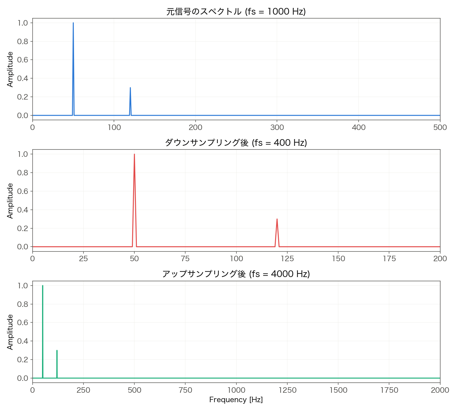
Both the 50 Hz and 120 Hz peaks are preserved across all resampled versions (visible in the figure above), confirming that the spectral content is faithfully maintained as long as the Nyquist condition is satisfied at the target rate.
Code 5: Verifying Bandpass (Sub-Nyquist) Sampling Numerically
We confirm that equation \((14)\) from the bandpass sampling section actually holds, by sampling two tones (22 MHz and 24 MHz) inside the \([20, 25]\) MHz band at \(f_s = 13\) MHz — inside the valid \(n=4\) band.
import numpy as np

# --- Generate a bandpass signal: two tones inside [20, 25] MHz ---
f1, f2 = 22e6, 24e6   # tone frequencies inside the band
fs = 13e6             # sub-Nyquist sampling rate (inside the n=4 band [12.5, 13.333] MHz)

duration = 20e-6      # 20 microseconds
t = np.arange(0, duration, 1 / fs)
x = np.sin(2 * np.pi * f1 * t) + 0.6 * np.sin(2 * np.pi * f2 * t)

# --- Theoretical alias frequency (same folding formula as equation (10)) ---
def alias(f, fs):
    return abs(f - round(f / fs) * fs)

a1, a2 = alias(f1, fs), alias(f2, fs)
print(f"Theoretical alias: {f1/1e6} MHz -> {a1/1e6:.3f} MHz, {f2/1e6} MHz -> {a2/1e6:.3f} MHz")

# --- Confirm the observed peaks via FFT ---
N = len(x)
X = np.fft.rfft(x)
freqs = np.fft.rfftfreq(N, 1 / fs)
mag = 2 / N * np.abs(X)

top_idx = np.argsort(mag)[::-1][:2]
for i in sorted(top_idx):
    print(f"Observed peak: f={freqs[i]/1e6:.4f} MHz, amplitude={mag[i]:.4f}")
Output:
Theoretical alias: 22.0 MHz -> 4.000 MHz, 24.0 MHz -> 2.000 MHz
Observed peak: f=2.0000 MHz, amplitude=0.6000
Observed peak: f=4.0000 MHz, amplitude=1.0000
The alias frequencies predicted by equation \((10)\) (22 MHz -> 4.0 MHz, 24 MHz -> 2.0 MHz) match the FFT-observed peaks exactly. The amplitudes also match the original coefficients (1.0 and 0.6) precisely, confirming that no information is lost even at the much lower rate \(f_s = 13\) MHz.
![Bandpass sampling: two tones in the [20, 25] MHz band, sampled at fs=13 MHz, map uniquely to 2 MHz and 4 MHz in baseband](/posts/20260430_sampling_theorem/bandpass_sampling.png)
Upsampling and Downsampling
Decimation (Downsampling)
Integer-ratio downsampling by factor \(M\) follows two mandatory steps:
- Anti-aliasing low-pass filter: cutoff at \(f_s / (2M)\)
- Keep every \(M\) -th sample: \(y[n] = x_{\text{filtered}}[Mn]\)
Skipping step 1 causes all energy above \(f_s/(2M)\)
to alias. scipy.signal.decimate automates both steps.
Interpolation (Upsampling)
Integer-ratio upsampling by factor \(L\) :
- Insert \(L-1\) zeros between consecutive samples
- Image-rejection LPF: cutoff \(f_s/(2L)\) , gain \(L\)
Zero insertion creates \(L-1\) spectral images that must be removed by the LPF. Without step 2, the upsampled signal has artificial high-frequency oscillations.
Polyphase Filtering
In production systems, resampling is implemented with polyphase filters. By decomposing the prototype LPF into \(L\) sub-filters (polyphase components), all multiplications with zero-valued samples are eliminated, reducing computational cost by a factor of \(L\) .
scipy.signal.resample_poly implements polyphase filtering and supports any rational ratio \(L/M\)
:
from scipy.signal import resample_poly

# 1000 Hz -> 441 Hz (L=441, M=1000), using x_orig from Code 4 above
x_poly = resample_poly(x_orig, 441, 1000)
print(f"Polyphase resample: {len(x_orig)} -> {len(x_poly)} samples")
Output:
Polyphase resample: 1000 -> 441 samples
The same mechanism underlies sample-rate conversion (SRC) between CD audio (44.1 kHz) and professional audio interfaces (48 kHz), e.g. resample_poly(x_44k, 160, 147). The internal details of the polyphase decomposition — Type-1 decomposition, computational savings via Noble identities, and so on — are covered in depth in
Multirate Signal Processing in Python
; this article stops at the point where the sampling theorem requires an anti-aliasing/image-rejection filter for any integer- or rational-ratio rate conversion.
Advanced Topic: Beyond Linear Reconstruction
The Nyquist-Shannon theorem covered in this article assumes perfect reconstruction via linear (sinc) interpolation of a band-limited signal. Recent research relaxes this assumption. Najaf and Ongie (2024), “Towards a Sampling Theory for Implicit Neural Representations” ( arXiv:2405.18410 ), presented at the 58th Asilomar Conference on Signals, Systems, and Computers, derive the number of samples needed to exactly recover a continuous-domain signal (image) from low-pass Fourier coefficients, under the assumption that the signal is well-approximated by a simple neural network (a single-hidden-layer ReLU implicit neural representation, or INR). Unlike the classical theorem’s linear-interpolation assumption, this line of work shows that exploiting nonlinear prior knowledge about the signal class (representability by an INR) can, in principle, achieve the same reconstruction accuracy from fewer samples. A parallel trend is visible in MRI reconstruction, where INR-based methods recover images from k-space data acquired at sub-Nyquist rates — a practical application that complements the classical linear sampling theory discussed throughout this article.
Summary
| Concept | Definition | Key Point |
|---|---|---|
| Sampling Theorem | \(f_s > 2f_{\max}\) | Necessary and sufficient for perfect reconstruction |
| Nyquist Frequency | \(f_N = f_s / 2\) | Maximum frequency the system can represent |
| Nyquist Rate | \(f_{NR} = 2f_{\max}\) | Minimum sampling frequency required by the signal |
| Alias Frequency | \(f_\text{alias} = \|f - \text{round}(f/f_s)\cdot f_s\|\) | Frequency at which an aliased component appears |
| Anti-Aliasing Filter | Analog LPF before ADC | Cutoff \(\leq f_s/2\) ; mandatory before downsampling |
| Decimation | AAF → keep every \(M\) -th sample | scipy.signal.decimate |
| Interpolation | Insert zeros → image-rejection LPF | scipy.signal.resample_poly |
| Bandpass Sampling | Eq. \((14)\) : \(2f_H/n \leq f_s \leq 2f_L/(n-1)\) | Can preserve information at \(f_s \ll 2f_H\) (SDR IF sampling) |
Understanding the sampling theorem is the foundation of any DSP system design. Pair this knowledge with Window Functions and PSD and Low-Pass Filter Design for a complete picture of the analog-to-digital signal processing pipeline.
Related Articles
- FFT: Theory and Python Implementation - Frequency analysis of discrete sampled signals; the FFT is inseparable from sampling theory.
- Window Functions and Power Spectral Density (PSD) - Spectral analysis after sampling, including windowing and the Welch PSD estimator.
- Low-Pass Filter Design and Comparison - Design of the anti-aliasing and image-rejection filters central to this article.
- Butterworth Filter Design and Python Implementation - In-depth design of the Butterworth filter — the most common choice for anti-aliasing.
- DTFT, DFT, and FFT: Putting the Hierarchy in Order - Connects the continuous-frequency representation of a sampled signal (DTFT) with its computable discrete forms (DFT/FFT).
- Signal Interpolation and Resampling - How the perfect reconstruction promised by the sampling theorem is realised in practice via sinc and polynomial interpolation.
- Z-Transform and Digital Filter Transfer Functions - The transfer-function framework that makes sampled discrete-time systems tractable.
- Discrete Cosine Transform (DCT) - The energy-compaction transform applied to sampled signals; the backbone of JPEG/MP3.
- Autocorrelation Function and Power Spectral Density - Periodicity detection and Wiener-Khinchin PSD computation on sampled discrete signals.
- Filter Design: Comprehensive Guide - End-to-end overview of filter design, including the anti-aliasing filter that this article motivates.
- Time-Frequency Analysis Guide - Bird’s-eye view of time-frequency methods applied to sampled signals.
- DSP x ML Roadmap - A meta-roadmap that places the sampling theorem as the entry point of the DSP-to-ML learning path.
- Discrete DSP Fundamentals Roadmap - Connects sampling, interpolation, DFT, Z-transform, autocorrelation, and DCT into a single discrete-DSP learning track. This article is its starting point.
- Multirate Signal Processing in Python: Decimation, Interpolation, and Polyphase Filters - Builds on the sampling theorem to change the sampling rate itself; the in-depth follow-up to this article’s up/down-sampling section.
References
- Shannon, C. E. (1949). “Communication in the Presence of Noise”. Proceedings of the IRE, 37(1), 10–21.
- Nyquist, H. (1928). “Certain Topics in Telegraph Transmission Theory”. Transactions of the AIEE, 47(2), 617–644.
- Oppenheim, A. V., & Schafer, R. W. (2009). Discrete-Time Signal Processing (3rd ed.). Prentice Hall.
- Proakis, J. G., & Manolakis, D. G. (2006). Digital Signal Processing (4th ed.). Prentice Hall.
- Najaf, M., & Ongie, G. (2024). “Towards a Sampling Theory for Implicit Neural Representations”. 58th Asilomar Conference on Signals, Systems, and Computers. arXiv:2405.18410
- SciPy Signal Processing documentation