Introduction
When designing and analyzing digital filters, working directly with difference equations quickly becomes cumbersome. Just as the Laplace transform converts differential equations into algebraic equations in the continuous-time domain, the Z-transform converts difference equations into algebraic equations and makes the theoretical treatment of digital filters dramatically simpler.
With the Z-transform, the following can be understood systematically:
- Deriving the transfer function \(H(z)\) of a digital filter
- Intuitively grasping filter characteristics from the placement of poles and zeros in the complex plane
- Expressing system stability conditions mathematically
- Computing frequency response by evaluating \(H(z)\) on the unit circle
This article progresses from the definition and basic properties of the Z-transform through inverse transforms, pole-zero plots, transfer functions and stability, and the connection to frequency response. Python implementations using scipy are provided throughout.
Reading about Butterworth filter design and FIR vs IIR filter comparison beforehand will deepen your understanding of this article.
Z-Transform Definition and Region of Convergence
Bilateral Z-Transform
The bilateral Z-transform of a discrete-time signal \(x[n]\) (\(n \in \mathbb{Z}\) ) is defined as:
\[X(z) = \mathcal{Z}\{x[n]\} = \sum_{n=-\infty}^{\infty} x[n]\, z^{-n} \tag{1}\]where \(z\) is a complex variable. Writing \(z = re^{j\omega}\) (\(r > 0\) ), equation \((1)\) expands to:
\[X(re^{j\omega}) = \sum_{n=-\infty}^{\infty} x[n]\, r^{-n} e^{-j\omega n} \tag{2}\]This has the same form as the Discrete-Time Fourier Transform (DTFT) of the signal \(x[n] r^{-n}\) . The Z-transform can therefore be viewed as a generalization of the DTFT to the entire complex plane.
Unilateral Z-Transform
When dealing with causal systems (\(x[n] = 0\) for \(n < 0\) ), the unilateral Z-transform is used:
\[X(z) = \sum_{n=0}^{\infty} x[n]\, z^{-n} \tag{3}\]Causal systems are standard in digital filter design; unless stated otherwise, we assume the unilateral Z-transform.
Region of Convergence (ROC)
The infinite series in equation \((1)\) does not necessarily converge for all values of \(z\) . The set of \(z\) values for which the Z-transform converges is called the Region of Convergence (ROC).
The ROC takes the form of an annular region \(r_1 < |z| < r_2\) centered at the origin. Key properties include:
- Finite-length signals: ROC is the entire complex plane except possibly \(z = 0\) or \(z = \infty\)
- Right-sided signals (non-zero only for \(n \geq 0\) ): ROC is \(|z| > r_1\) (outside some radius)
- Left-sided signals (non-zero only for \(n \leq 0\) ): ROC is \(|z| < r_2\) (inside some radius)
- The ROC never contains poles
As an example, compute the Z-transform of \(x[n] = a^n u[n]\) (\(u[n]\) is the unit step function):
\[X(z) = \sum_{n=0}^{\infty} a^n z^{-n} = \sum_{n=0}^{\infty} (az^{-1})^n = \frac{1}{1 - az^{-1}} = \frac{z}{z - a} \tag{4}\]This series converges when \(|az^{-1}| < 1\) , i.e., \(|z| > |a|\) . The ROC is the exterior region \(|z| > |a|\) .
Key Properties of the Z-Transform
Linearity
\[\mathcal{Z}\{\alpha x_1[n] + \beta x_2[n]\} = \alpha X_1(z) + \beta X_2(z) \tag{5}\]The ROC contains at least the intersection \(\text{ROC}_1 \cap \text{ROC}_2\) .
Time Shift
\[\mathcal{Z}\{x[n - k]\} = z^{-k} X(z) \tag{6}\]Proof: Substitute into the definition and set \(m = n - k\) :
\[\sum_{n=-\infty}^{\infty} x[n-k] z^{-n} = \sum_{m=-\infty}^{\infty} x[m] z^{-(m+k)} = z^{-k} \sum_{m=-\infty}^{\infty} x[m] z^{-m} = z^{-k} X(z)\]This property is essential for converting difference equations into algebraic equations in the Z-domain. The factor \(z^{-1}\) acts as a “one-sample delay” operator.
Convolution Theorem
\[\mathcal{Z}\{x_1[n] * x_2[n]\} = X_1(z) \cdot X_2(z) \tag{7}\]Convolution in the time domain becomes multiplication in the Z-domain. This means that filtering (convolution of input signal with impulse response) is expressed as multiplication of transfer functions.
Time Reversal
\[\mathcal{Z}\{x[-n]\} = X(z^{-1}) \tag{8}\]Z-Domain Differentiation (Multiplication Property)
\[\mathcal{Z}\{n \cdot x[n]\} = -z \frac{d}{dz} X(z) \tag{9}\]Initial Value and Final Value Theorems
For causal signals, the following theorems hold.
Initial Value Theorem:
\[x[0] = \lim_{z \to \infty} X(z) \tag{10}\]Final Value Theorem:
\[\lim_{n \to \infty} x[n] = \lim_{z \to 1} (z-1) X(z) \tag{11}\]The final value theorem is useful for finding the steady-state output of a system using only Z-domain algebra, without simulating in the time domain. It applies only when all poles of \((z-1)X(z)\) lie strictly inside the unit circle.
Common Transform Pairs
| \(x[n]\) | \(X(z)\) | ROC |
|---|---|---|
| \(\delta[n]\) | \(1\) | All \(z\) |
| \(u[n]\) | \(\dfrac{z}{z-1}\) | \(\|z\| > 1\) |
| \(a^n u[n]\) | \(\dfrac{z}{z-a}\) | \(\|z\| > \|a\|\) |
| \(n u[n]\) | \(\dfrac{z}{(z-1)^2}\) | \(\|z\| > 1\) |
| \(\cos(\omega_0 n) u[n]\) | \(\dfrac{z(z-\cos\omega_0)}{z^2 - 2z\cos\omega_0 + 1}\) | \(\|z\| > 1\) |
| \(r^n \cos(\omega_0 n) u[n]\) | \(\dfrac{z(z - r\cos\omega_0)}{z^2 - 2rz\cos\omega_0 + r^2}\) | \(\|z\| > r\) |
Inverse Z-Transform
Partial Fraction Expansion Method
The most widely used method. Express \(X(z)\) as a rational function and decompose it into terms that match known transform pairs.
The standard procedure is to expand \(X(z)/z\) (or \(H(z)/z\) ) into partial fractions.
Example: Compute the inverse Z-transform of the following.
\[X(z) = \frac{z^2}{(z - 0.5)(z - 0.8)}, \quad |z| > 0.8 \tag{12}\]Expand \(X(z)/z\) in partial fractions:
\[\frac{X(z)}{z} = \frac{z}{(z-0.5)(z-0.8)} = \frac{A}{z-0.5} + \frac{B}{z-0.8}\] \[A = \left.\frac{z}{z-0.8}\right|_{z=0.5} = \frac{0.5}{0.5-0.8} = -\frac{5}{3}\] \[B = \left.\frac{z}{z-0.5}\right|_{z=0.8} = \frac{0.8}{0.8-0.5} = \frac{8}{3}\]Therefore:
\[X(z) = -\frac{5}{3}\cdot\frac{z}{z-0.5} + \frac{8}{3}\cdot\frac{z}{z-0.8}\]Since the ROC is \(|z| > 0.8\) (right-sided signal):
\[x[n] = \left(-\frac{5}{3}(0.5)^n + \frac{8}{3}(0.8)^n\right)u[n] \tag{13}\]Power Series Expansion (Long Division)
Expand \(X(z)\) as a power series in \(z^{-1}\) :
\[X(z) = x[0] + x[1]z^{-1} + x[2]z^{-2} + \cdots \tag{14}\]Performing long division of the numerator by the denominator yields the coefficients directly. This is convenient for FIR filters and numerical verification.
Example: Expand \(X(z) = \dfrac{1 + z^{-1}}{1 - 0.5z^{-1}}\) .
Long division gives \(x[0]=1,\; x[1]=1.5,\; x[2]=0.75,\; x[3]=0.375, \ldots\) , which yields \(x[n] = \delta[n] + 1.5(0.5)^{n-1}u[n-1]\) .
Residue Method (Cauchy Integral Formula)
\[x[n] = \frac{1}{2\pi j} \oint_C X(z) z^{n-1} dz = \sum_k \text{Res}\left[X(z)z^{n-1}, z_k\right] \tag{15}\]where \(C\) is a counterclockwise closed contour inside the ROC and \(z_k\) are poles enclosed by \(C\) . This is important for theoretical analysis, but in practice the partial fraction method is more straightforward.
Poles, Zeros, and the Z-Plane
Definitions
For a rational function \(X(z) = N(z)/D(z)\) where \(N\) and \(D\) are polynomials:
- Values \(z_0\) where \(N(z_0) = 0\) : zeros
- Values \(z_p\) where \(D(z_p) = 0\) : poles
A rational function with numerator degree \(M\) and denominator degree \(N\) has \(M\) zeros and \(N\) poles (counting zeros/poles at infinity).
Pole-Zero Plot
Plotting poles as × and zeros as ○ on the complex plane (z-plane) produces a pole-zero plot. This is the single most important tool for visually grasping the characteristics of a digital filter.
The magnitude of the filter frequency response corresponds to \(|H(z)|\) as \(z\) sweeps along the unit circle \(z = e^{j\omega}\) :
- Zero near the unit circle: gain decreases (notch) near that angular frequency
- Pole near the unit circle: gain increases (peak) near that angular frequency
- Pole on or outside the unit circle: system is unstable
Stability Condition
An LTI (Linear Time-Invariant) discrete-time system is BIBO stable if and only if:
\[\text{all poles } z_k \text{ lie strictly inside the unit circle}: \quad |z_k| < 1 \quad \forall k \tag{16}\]This has an intuitive explanation. The time-domain component corresponding to pole \(z_k = r_k e^{j\theta_k}\) is proportional to \(r_k^n e^{j\theta_k n}\) . If \(r_k < 1\) , this decays as \(n \to \infty\) ; if \(r_k > 1\) , it diverges.
Transfer Function and Difference Equations
Definition of the Transfer Function
The transfer function \(H(z)\) of a linear time-invariant system is defined as the ratio of the Z-transform of the output \(Y(z)\) to the Z-transform of the input \(X(z)\) :
\[H(z) = \frac{Y(z)}{X(z)} \tag{17}\]By the convolution theorem, \(Y(z) = H(z) X(z)\) , so \(H(z)\) is the Z-transform of the impulse response \(h[n]\) .
From Difference Equation to Transfer Function
A general \(N\) -th order difference equation is:
\[y[n] = -\sum_{k=1}^{N} a_k\, y[n-k] + \sum_{k=0}^{M} b_k\, x[n-k] \tag{18}\]Taking the Z-transform of both sides and applying the time-shift property \(\mathcal{Z}\{y[n-k]\} = z^{-k} Y(z)\) :
\[Y(z) = -\sum_{k=1}^{N} a_k z^{-k} Y(z) + \sum_{k=0}^{M} b_k z^{-k} X(z)\]Rearranging:
\[H(z) = \frac{Y(z)}{X(z)} = \frac{\sum_{k=0}^{M} b_k z^{-k}}{1 + \sum_{k=1}^{N} a_k z^{-k}} \tag{19}\]This is the general form of the IIR filter transfer function.
FIR and IIR Filters in the Z-Domain
FIR filters (Finite Impulse Response) have no feedback (all \(a_k = 0\) ):
\[H_{\text{FIR}}(z) = \sum_{k=0}^{M} b_k z^{-k} = b_0 + b_1 z^{-1} + \cdots + b_M z^{-M} \tag{20}\]This is a polynomial with no poles (except at the origin). FIR filters are designed using zeros only.
IIR filters (Infinite Impulse Response) have feedback (\(a_k \neq 0\) ):
\[H_{\text{IIR}}(z) = \frac{B(z)}{A(z)} = \frac{\sum_{k=0}^{M} b_k z^{-k}}{1 + \sum_{k=1}^{N} a_k z^{-k}} \tag{21}\]IIR filters have both poles and zeros. They can realize steep frequency responses with fewer coefficients, but require careful stability management. See FIR and IIR Filter Comparison for details.
Pole-Zero Form
Expressing the transfer function as a product of poles and zeros:
\[H(z) = b_0 \frac{\prod_{k=1}^{M} (1 - q_k z^{-1})}{\prod_{k=1}^{N} (1 - p_k z^{-1})} \tag{22}\]where \(q_k\) are zeros and \(p_k\) are poles. This representation corresponds directly to the pole-zero plot and offers an intuitive understanding of filter characteristics.
Stability Analysis
Stable, Unstable, and Marginally Stable Systems
| Pole location | System behavior | Classification |
|---|---|---|
| \(\|p_k\| < 1\) (all poles) | Impulse response decays | Stable |
| \(\|p_k\| = 1\) (simple pole) | Impulse response oscillates indefinitely | Marginally stable |
| \(\|p_k\| > 1\) (any pole) | Impulse response diverges | Unstable |
Second-Order Sections and Numerical Stability
Implementing a high-order IIR filter directly can cause poles to migrate outside the unit circle due to finite-precision arithmetic errors. To prevent this, IIR filters are standardly decomposed into and implemented as Second-Order Sections (SOS):
\[H(z) = \prod_{k=1}^{K} H_k(z), \quad H_k(z) = \frac{b_{k,0} + b_{k,1}z^{-1} + b_{k,2}z^{-2}}{1 + a_{k,1}z^{-1} + a_{k,2}z^{-2}} \tag{23}\]scipy.signal.butter(..., output='sos') returns coefficients in this form.
Frequency Response from Poles and Zeros
Evaluating on the Unit Circle
The frequency response of a digital filter is obtained by evaluating the transfer function \(H(z)\) on the unit circle \(z = e^{j\omega}\) (\(\omega \in [-\pi, \pi]\) ):
\[H(e^{j\omega}) = H(z)\big|_{z=e^{j\omega}} = \sum_{n=-\infty}^{\infty} h[n]\, e^{-j\omega n} \tag{24}\]This coincides with the DTFT. The Fast Fourier Transform (FFT) computes discrete samples of this.
Geometric Interpretation from Poles and Zeros
Substituting \(z = e^{j\omega}\) into equation \((22)\) :
\[H(e^{j\omega}) = b_0 \frac{\prod_{k=1}^{M} (e^{j\omega} - q_k)}{\prod_{k=1}^{N} (e^{j\omega} - p_k)} \tag{25}\]Each factor can be interpreted as a “vector” in the complex plane:
- \(|e^{j\omega} - q_k|\) : distance from the point \(e^{j\omega}\) on the unit circle to zero \(q_k\)
- \(|e^{j\omega} - p_k|\) : distance from the point \(e^{j\omega}\) on the unit circle to pole \(p_k\)
Therefore:
\[|H(e^{j\omega})| = |b_0| \frac{\prod_k |e^{j\omega} - q_k|}{\prod_k |e^{j\omega} - p_k|} \tag{26}\] \[\angle H(e^{j\omega}) = \sum_k \angle(e^{j\omega} - q_k) - \sum_k \angle(e^{j\omega} - p_k) \tag{27}\]From this geometric interpretation:
- A pole close to the unit circle at some angular frequency → denominator is small → gain increases (peak)
- A zero close to the unit circle at some angular frequency → numerator is small → gain decreases (notch)
- A zero on the unit circle at some angular frequency → \(|H| = 0\) (complete rejection)
For the theoretical treatment of phase characteristics, see also Phase and Group Delay Analysis .
Python Implementation
Importing Libraries
import numpy as np
import matplotlib.pyplot as plt
from scipy.signal import butter, freqz, tf2zpk, zpk2tf, sosfilt
Pole-Zero Plot Function (zplane)
def zplane(b, a, ax=None, title="Pole-Zero Plot"):
    """
    Draw a pole-zero plot for a digital filter.

    Parameters
    ----------
    b : array_like
        Numerator coefficients (b[0] + b[1]*z^-1 + ...)
    a : array_like
        Denominator coefficients (a[0] + a[1]*z^-1 + ...)
    ax : matplotlib Axes, optional
        Target Axes. Creates a new figure if None.
    title : str
        Plot title

    Returns
    -------
    zeros : ndarray
        Array of zeros
    poles : ndarray
        Array of poles
    """
    if ax is None:
        fig, ax = plt.subplots(figsize=(6, 6))

    # Compute poles and zeros
    zeros, poles, gain = tf2zpk(b, a)

    # Draw unit circle
    theta = np.linspace(0, 2 * np.pi, 512)
    ax.plot(np.cos(theta), np.sin(theta), "k--", linewidth=0.8, alpha=0.5, label="Unit Circle")

    # Real and imaginary axes
    ax.axhline(0, color="k", linewidth=0.5, alpha=0.4)
    ax.axvline(0, color="k", linewidth=0.5, alpha=0.4)

    # Zeros (circles)
    ax.scatter(zeros.real, zeros.imag, s=80, marker="o", facecolors="none",
               edgecolors="blue", linewidths=1.5, zorder=5, label=f"Zeros ({len(zeros)})")

    # Poles (crosses)
    ax.scatter(poles.real, poles.imag, s=80, marker="x",
               color="red", linewidths=1.5, zorder=5, label=f"Poles ({len(poles)})")

    # Axis settings
    ax.set_xlabel("Real Part")
    ax.set_ylabel("Imaginary Part")
    ax.set_title(title)
    ax.set_aspect("equal")
    ax.legend(fontsize=8)
    ax.grid(True, alpha=0.3)

    # Auto-set limits to accommodate unit circle
    # Guard against np.max on an empty array when there are no zeros or no poles
    candidates = [1.5]
    if len(poles) > 0:
        candidates.append(np.max(np.abs(poles)) * 1.2)
    if len(zeros) > 0:
        candidates.append(np.max(np.abs(zeros)) * 1.2)
    lim = max(candidates)
    ax.set_xlim(-lim, lim)
    ax.set_ylim(-lim, lim)

    return zeros, poles
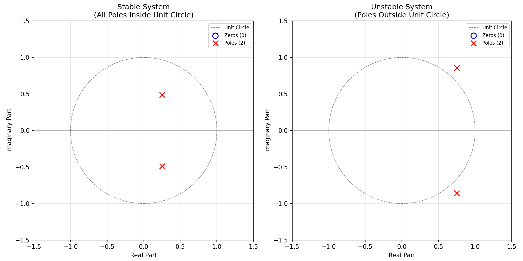
Comparing Stable and Unstable Systems
# --- Stable system (all poles inside unit circle) ---
b_stable = np.array([1.0])
a_stable = np.array([1.0, -0.5, 0.3])   # poles: |p| < 1

# --- Unstable system (poles outside unit circle) ---
b_unstable = np.array([1.0])
a_unstable = np.array([1.0, -1.5, 1.3]) # poles: |p| > 1

fig, axes = plt.subplots(1, 2, figsize=(12, 6))
z_s, p_s = zplane(b_stable, a_stable, ax=axes[0],
                  title="Stable System\n(All Poles Inside Unit Circle)")
z_u, p_u = zplane(b_unstable, a_unstable, ax=axes[1],
                  title="Unstable System\n(Poles Outside Unit Circle)")

print(f"Stable system poles:   {np.roots(a_stable)}")
print(f"  Magnitudes: {np.abs(np.roots(a_stable))}")
print(f"Unstable system poles: {np.roots(a_unstable)}")
print(f"  Magnitudes: {np.abs(np.roots(a_unstable))}")

plt.tight_layout()
plt.show()
Actual output from running the code above (NumPy 2.4.2 / SciPy 1.18.0):
Stable system poles:   [0.25+0.48733972j 0.25-0.48733972j]
  Magnitudes: [0.54772256 0.54772256]
Unstable system poles: [0.75+0.8587782j  0.75-0.8587782j]
  Magnitudes: [1.14017543 1.14017543]
Pitfall: For a 2nd-order denominator \(z^2 + a_1 z + a_2\)
, the squared magnitude of a complex-conjugate pole pair \(|p_k|^2\)
equals the constant term \(a_2\)
by Vieta’s formulas. Naively setting a_unstable = [1.0, -1.5, 0.9] gives \(|p_k| = \sqrt{0.9} \approx 0.949 < 1\)
— the intended “unstable” example is actually stable. To build a genuine unstable example with a complex-conjugate pole pair, the denominator’s constant term \(a_2\)
itself must exceed 1 (here \(a_2 = 1.3\)
, giving \(|p_k| = \sqrt{1.3} \approx 1.140\)
as intended). This is a typical case where choosing coefficients without deriving them leads to a sign or magnitude error.
Here is the pole-zero plot actually generated by the code above:
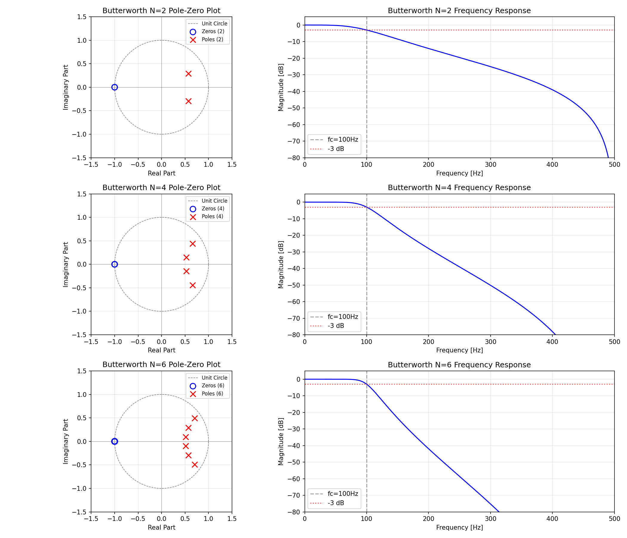
Butterworth Filter Pole-Zero Analysis
# Butterworth low-pass filter (cutoff 100 Hz, sampling 1000 Hz)
fs = 1000   # Hz
fc = 100    # Hz
orders = [2, 4, 6]

fig, axes = plt.subplots(len(orders), 2, figsize=(14, 4 * len(orders)))

for i, N in enumerate(orders):
    # Design in SOS form
    sos = butter(N, fc, fs=fs, output='sos')
    # Convert to transfer function form
    b, a = butter(N, fc, fs=fs, output='ba')

    # Left column: pole-zero plot
    zplane(b, a, ax=axes[i, 0], title=f"Butterworth N={N} Pole-Zero Plot")

    # Right column: frequency response
    w, h = freqz(b, a, worN=4096, fs=fs)
    axes[i, 1].plot(w, 20 * np.log10(np.abs(h) + 1e-12), "b", linewidth=1.5)
    axes[i, 1].axvline(fc, color="gray", linestyle="--", alpha=0.7, label=f"fc={fc}Hz")
    axes[i, 1].axhline(-3, color="red", linestyle=":", alpha=0.7, label="-3 dB")
    axes[i, 1].set_xlim(0, fs / 2)
    axes[i, 1].set_ylim(-80, 5)
    axes[i, 1].set_xlabel("Frequency [Hz]")
    axes[i, 1].set_ylabel("Magnitude [dB]")
    axes[i, 1].set_title(f"Butterworth N={N} Frequency Response")
    axes[i, 1].legend()
    axes[i, 1].grid(True, alpha=0.3)

plt.tight_layout()
plt.show()
Actual output from running the code above (poles/zeros rounded to 4 decimal places):
N=2: poles  = [0.5715+0.2936j, 0.5715-0.2936j]
     |poles| = [0.6425, 0.6425]
     zeros  = [-1.0000, -1.0000]

N=4: poles  = [0.6605+0.4433j, 0.6605-0.4433j, 0.5243+0.1458j, 0.5243-0.1458j]
     |poles| = [0.7954, 0.7954, 0.5442, 0.5442]
     zeros  = [-1.0002+0.0000j, -1.0000+0.0002j, -1.0000-0.0002j, -0.9998+0.0000j]

N=6: poles  = [0.7022+0.4928j, 0.7022-0.4928j, 0.5715+0.2936j, 0.5715-0.2936j, 0.5160+0.0970j, 0.5160-0.0970j]
     |poles| = [0.8579, 0.8579, 0.6425, 0.6425, 0.5251, 0.5251]
     zeros  = [-1.0035+0.0020j, -1.0035-0.0020j, -1.0000+0.0041j, -1.0000-0.0041j, -0.9965+0.0020j, -0.9965-0.0020j]
At every order, the zeros cluster near \(z \approx -1\) (the Nyquist frequency \(f_s/2\) ) — a hallmark of the Butterworth low-pass design, which places an \(N\) -th order zero at \(z=-1\) . The pole magnitudes, meanwhile, grow closer to the unit circle as the order increases: from a maximum of \(0.6425\) at \(N=2\) to \(0.8579\) at \(N=6\) . This is the numerical signature of needing poles ever closer to the unit circle to realize a steeper roll-off, and it is exactly why higher-order Butterworth filters are more susceptible to finite-precision numerical instability (the reason SOS decomposition is recommended).
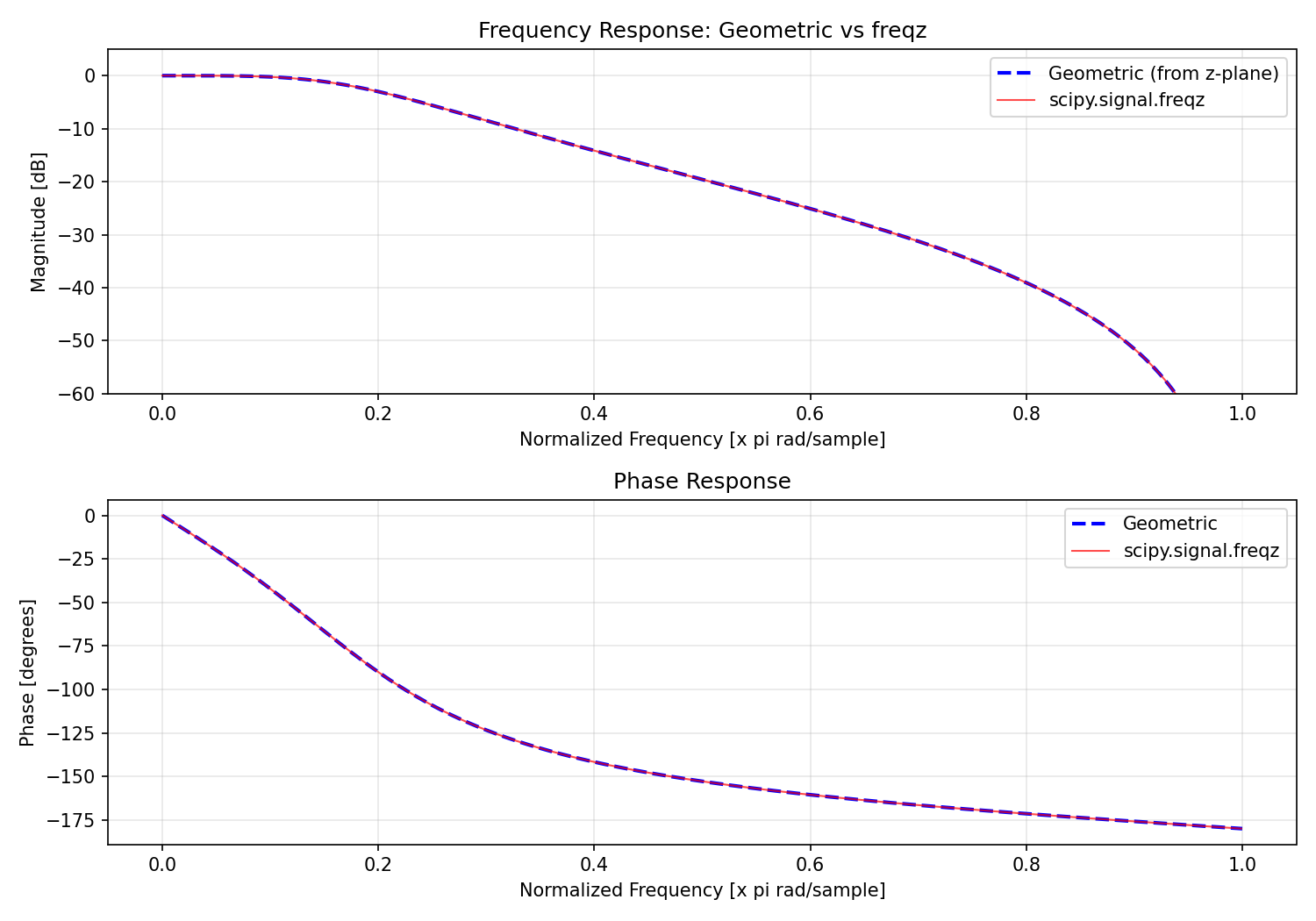
Frequency Response from Poles and Zeros (Geometric Visualization)
def freq_response_from_zpk(zeros, poles, gain, omega_range=None):
    """
    Compute magnitude and phase of the frequency response
    geometrically from poles and zeros.

    Parameters
    ----------
    zeros : array_like
        Array of zeros (complex)
    poles : array_like
        Array of poles (complex)
    gain : float
        Gain constant
    omega_range : array_like, optional
        Angular frequencies to evaluate (rad/sample)

    Returns
    -------
    omega : ndarray
        Angular frequencies
    H_mag : ndarray
        Magnitude response
    H_phase : ndarray
        Phase response [rad]
    """
    if omega_range is None:
        omega_range = np.linspace(0, np.pi, 1024)

    H_mag = np.ones(len(omega_range)) * np.abs(gain)
    H_phase = np.zeros(len(omega_range))

    for idx in range(len(omega_range)):
        z = np.exp(1j * omega_range[idx])

        # Product of distances from zeros
        for q in zeros:
            H_mag[idx] *= np.abs(z - q)
            H_phase[idx] += np.angle(z - q)

        # Product of distances from poles
        for p in poles:
            H_mag[idx] /= np.abs(z - p)
            H_phase[idx] -= np.angle(z - p)

    return omega_range, H_mag, H_phase


# Example: 2nd-order Butterworth LPF via geometric computation
b, a = butter(2, 0.2)   # digital cutoff at 0.2π (normalized)
zeros, poles, gain = tf2zpk(b, a)

omega, H_mag, H_phase = freq_response_from_zpk(zeros, poles, gain)

# Compare with scipy.signal.freqz
w, h = freqz(b, a, worN=1024)

fig, axes = plt.subplots(2, 1, figsize=(10, 7))

axes[0].plot(omega / np.pi, 20 * np.log10(H_mag + 1e-12), "b--",
             linewidth=2, label="Geometric (from z-plane)")
axes[0].plot(w / np.pi, 20 * np.log10(np.abs(h) + 1e-12), "r",
             linewidth=1, alpha=0.7, label="scipy.signal.freqz")
axes[0].set_xlabel("Normalized Frequency [× π rad/sample]")
axes[0].set_ylabel("Magnitude [dB]")
axes[0].set_title("Frequency Response: Geometric vs freqz")
axes[0].legend()
axes[0].grid(True, alpha=0.3)
axes[0].set_ylim(-60, 5)

axes[1].plot(omega / np.pi, np.degrees(np.unwrap(H_phase)), "b--",
             linewidth=2, label="Geometric")
axes[1].plot(w / np.pi, np.degrees(np.unwrap(np.angle(h))), "r",
             linewidth=1, alpha=0.7, label="scipy.signal.freqz")
axes[1].set_xlabel("Normalized Frequency [× π rad/sample]")
axes[1].set_ylabel("Phase [degrees]")
axes[1].set_title("Phase Response")
axes[1].legend()
axes[1].grid(True, alpha=0.3)

plt.tight_layout()
plt.show()
Actual output from running the code above:
b = [0.06745527 0.13491055 0.06745527]
a = [ 1.         -1.1429805   0.4128016 ]
zeros = [-0.99999999 -1.00000001]
poles = [0.57149025+0.2935992j 0.57149025-0.2935992j]
gain  = 0.06745527388907191

Max magnitude error (geometric vs freqz): 8.27e-04 (peaks near ω ≈ 0.242π)
The error is not at machine precision (\(\sim 10^{-16}\)
) but rather \(10^{-4}\)
, because freq_response_from_zpk sequentially multiplies/adds magnitudes and angles for each pole and zero inside a loop, whereas scipy.signal.freqz uses a numerically stable direct polynomial evaluation. Both compute the same \(H(e^{j\omega})\)
in theory, but the two computational paths accumulate floating-point error differently, and the discrepancy peaks at an angular frequency (\(\omega \approx 0.242\pi\)
) that happens to lie relatively close to the poles and zeros. This is negligible in practice, but for high-order filters with many poles and zeros such loop-based errors can accumulate — implementations should prefer freqz (or an SOS decomposition) over a hand-rolled loop.
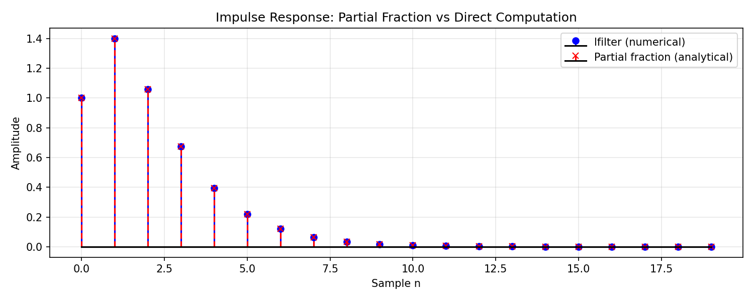
Inverse Z-Transform via Partial Fractions (Numerical Verification)
from scipy.signal import residuez

# H(z) = (1 + 0.5z^-1) / (1 - 0.9z^-1 + 0.2z^-2)
b = np.array([1.0, 0.5])
a = np.array([1.0, -0.9, 0.2])

# residuez returns H(z) = sum(r_k / (1 - p_k z^-1)) + k
r, p, k = residuez(b, a)

print("Partial fraction expansion: H(z) = sum(r_k / (1 - p_k * z^-1)) + k(z)")
for i, (ri, pi) in enumerate(zip(r, p)):
    print(f"  r[{i}] = {ri:.4f},  p[{i}] = {pi:.4f}  (|p| = {abs(pi):.4f})")
print(f"  Direct term k = {k}")

# Inverse Z-transform (analytical impulse response)
N = 20
n = np.arange(N)
h_analytical = np.zeros(N, dtype=complex)
for ri, pi in zip(r, p):
    h_analytical += ri * pi**n
h_analytical = h_analytical.real

# Compare with numerical computation via scipy.signal.lfilter
from scipy.signal import lfilter, unit_impulse
impulse = unit_impulse(N)
h_numerical = lfilter(b, a, impulse)

fig, ax = plt.subplots(figsize=(10, 4))
ax.stem(n, h_numerical, linefmt="b-", markerfmt="bo", basefmt="k-",
        label="lfilter (numerical)")
ax.stem(n, h_analytical, linefmt="r--", markerfmt="rx", basefmt="k-",
        label="Partial fraction (analytical)")
ax.set_xlabel("Sample n")
ax.set_ylabel("Amplitude")
ax.set_title("Impulse Response: Partial Fraction vs Direct Computation")
ax.legend()
ax.grid(True, alpha=0.3)
plt.tight_layout()
plt.show()

print(f"\nMax error: {np.max(np.abs(h_numerical - h_analytical)):.2e}")
Actual output from running the code above:
Partial fraction expansion: H(z) = sum(r_k / (1 - p_k * z^-1)) + k(z)
  r[0] = -9.0000,  p[0] = 0.4000  (|p| = 0.4000)
  r[1] = 10.0000,  p[1] = 0.5000  (|p| = 0.5000)
  Direct term k = []

Max error: 2.22e-16
residuez returned the partial fraction expansion
\(
H(z) = \dfrac{-9}{1 - 0.4z^{-1}} + \dfrac{10}{1 - 0.5z^{-1}}
\)
The direct term k is an empty array because the numerator degree (1) is strictly less than the denominator degree (2) — a strictly proper rational function; a direct polynomial term appears only when the numerator degree is greater than or equal to the denominator degree. The maximum error between the analytical solution and lfilter’s numerical computation is \(2.22 \times 10^{-16}\)
, exactly the double-precision floating-point rounding limit (machine epsilon \(\approx 2.22 \times 10^{-16}\)
) — confirming the two are theoretically identical.
Interconversion: Transfer Function, SOS, and ZPK Forms
from scipy.signal import tf2sos, sos2tf, zpk2sos

# 4th-order Butterworth in each representation
b, a = butter(4, 0.3)

# BA → ZPK
zeros, poles, gain = tf2zpk(b, a)

# ZPK → BA (round-trip)
b_r, a_r = zpk2tf(zeros, poles, gain)

# BA → SOS
sos = tf2sos(b, a)

# SOS → BA
b_sos, a_sos = sos2tf(sos)

print("=== 4th-Order Butterworth Filter: Representation Formats ===")
print(f"\nBA form (b): {b}")
print(f"BA form (a): {a}")
print(f"\nPoles: {poles}")
print(f"Zeros: {zeros}")
print(f"Gain:  {gain:.6f}")
print(f"\nSOS form:\n{sos}")

# Verify stability (all pole magnitudes < 1)
print(f"\nAll pole magnitudes (must all be < 1 for stability):")
for i, pol in enumerate(poles):
    print(f"  p[{i}] = {pol:.4f},  |p| = {abs(pol):.4f} {'OK' if abs(pol) < 1 else 'UNSTABLE'}")
Actual output from running the code above:
=== 4th-Order Butterworth Filter: Representation Formats ===

BA form (b): [0.01856301 0.07425204 0.11137806 0.07425204 0.01856301]
BA form (a): [ 1.         -1.57039885  1.27561332 -0.48440337  0.07619706]

Poles: [0.4488+0.5707j 0.4488-0.5707j 0.3364+0.1772j 0.3364-0.1772j]
Zeros: [-1.0002+0.0000j -1.0000+0.0002j -1.0000-0.0002j -0.9998+0.0000j]
Gain:  0.018563

SOS form:
[[ 0.01856301  0.03712602  0.01856301  1.         -0.67274091  0.1445352 ]
 [ 1.          2.00000004  0.99999999  1.         -0.89765794  0.5271869 ]]

All pole magnitudes (must all be < 1 for stability):
  p[0] = 0.4488+0.5707j,  |p| = 0.7261 OK
  p[1] = 0.4488-0.5707j,  |p| = 0.7261 OK
  p[2] = 0.3364+0.1772j,  |p| = 0.3802 OK
  p[3] = 0.3364-0.1772j,  |p| = 0.3802 OK
The round-trip error for BA→ZPK→BA is at most \(1.33 \times 10^{-15}\)
, and for BA→SOS→BA at most \(1.55 \times 10^{-15}\)
— both within double-precision rounding error, confirming the conversions are exact. Each SOS row is ordered \(b_{k,0}, b_{k,1}, b_{k,2}, 1, a_{k,1}, a_{k,2}\)
(the output convention of scipy.signal.tf2sos): the first row’s denominator \(1 - 0.6727z^{-1} + 0.1445z^{-2}\)
corresponds to the pole pair \(0.3364 \pm 0.1772j\)
(\(|p|=0.3802\)
), and the second row’s denominator \(1 - 0.8977z^{-1} + 0.5272z^{-2}\)
corresponds to the pole pair \(0.4488 \pm 0.5707j\)
(\(|p|=0.7261\)
).
Recent Research: Differentiable All-pole Filters and Machine Learning
The idea at the core of this article — constraining poles to lie inside the unit circle to guarantee BIBO stability (equation \((16)\) ) — also plays a central role in recent neural audio signal processing research.
A 2024 paper presented at DAFx (International Conference on Digital Audio Effects), “Differentiable All-pole Filters for Time-varying Audio Systems” (Yu, Mitcheltree, Carson, Bilbao, Reiss, & Fazekas, 2024, arXiv:2404.07970 ), reformulates the pole parameters of the all-pole filter discussed in this article (a special case of an IIR filter, \(H(z) = 1/A(z)\) ) so that they can be learned directly via gradient descent using automatic differentiation (e.g., PyTorch).
Training a time-varying all-pole filter with automatic differentiation traditionally required unrolling the recursive difference equation \(y[n] = x[n] - \sum_k a_k y[n-k]\) step by step in time, which is computationally expensive and prone to vanishing/exploding gradients. The paper proposes a method for backpropagating gradients through the all-pole filter itself, sidestepping the limitations of existing approaches such as frequency-sampling approximations.
The treatment of stability connects directly to this article’s content: if training pushes a pole outside the unit circle (\(|p_k| \geq 1\) ), the stability condition of equation \((16)\) is violated and the filter diverges. For this reason, work in this area widely adopts parameterizations that constrain the pole radius to \(|p_k| < 1\) using activation functions such as \(\tanh\) — precisely the stability condition derived in this article. It is a striking example of the classical Z-transform framework being embedded directly into a modern deep-learning pipeline for neural modeling of audio effects and synthesizers.
Summary
This article provided a systematic treatment of the Z-transform and its applications.
| Topic | Key Point |
|---|---|
| Z-transform definition | \(X(z) = \sum x[n] z^{-n}\) . Always specify the ROC. |
| Time-shift property | \(z^{-1}\) corresponds to a one-sample delay. Converts difference equations to algebra. |
| Convolution theorem | Time-domain convolution ↔ Z-domain multiplication. Filtering as \(Y = HX\) . |
| Inverse Z-transform | Partial fraction expansion is the practical approach. |
| Poles and zeros | Poles as ×, zeros as ○ plotted on the complex plane. |
| Stability | All poles inside the unit circle (\(\|p_k\| < 1\) ). |
| Transfer function | \(H(z) = B(z)/A(z)\) . One-to-one correspondence with difference equations. |
| Frequency response | \(H(e^{j\omega}) = H(z)\big\|_{z=e^{j\omega}}\) (on unit circle). |
| Geometric interpretation | Gain computed as product/quotient of distances from poles and zeros. |
The Z-transform is the cornerstone of digital signal processing theory. Once you can quickly assess filter characteristics just by examining the pole-zero placement, your understanding of filter design will deepen considerably.
Related Articles
- Fast Fourier Transform (FFT): How It Works and Python Implementation — Foundation of frequency analysis. Restricting the Z-transform to the unit circle gives the DTFT; its discrete samples give the DFT/FFT.
- Butterworth Filter Design: Principles and Python Implementation — A leading example of IIR filter design. The pole-zero plot and transfer function knowledge from this article applies directly.
- FIR and IIR Filter Comparison — Explains the Z-domain difference between FIR (all-zero filter) and IIR (has poles).
- Phase and Group Delay Analysis — Derives group delay from the phase of \(H(e^{j\omega})\) and analyzes the time-domain distortion of filters.
- DTFT, DFT, and FFT: Putting the Hierarchy in Order — Positions the DTFT as the Z-transform on the unit circle and the DFT/FFT as its discrete samples.
- Sampling Theorem and Aliasing — The continuous-to-discrete bridge that the Z-transform presupposes.
- Signal Interpolation and Resampling — A concrete example of designing interpolation / resampling filters as Z-domain transfer functions.
- Filter Design: Comprehensive Guide — Hub view of filter design starting from Z-domain pole-zero placement.
- Time-Frequency Analysis Guide — Organises time-frequency representations derived from the Z-transform.
- DSP x ML Roadmap — Meta-roadmap placing the Z-transform in the DSP-to-ML curriculum.
- Discrete DSP Fundamentals Roadmap — A hub bundling sampling, interpolation, DFT, Z-transform, autocorrelation, and DCT. The Z-transform sits at the core of mathematical operations on discrete-time systems.
References
- Oppenheim, A. V., & Schafer, R. W. (2009). Discrete-Time Signal Processing (3rd ed.). Prentice Hall.
- Proakis, J. G., & Manolakis, D. G. (2006). Digital Signal Processing: Principles, Algorithms, and Applications (4th ed.). Prentice Hall.
- Antoniou, A. (2005). Digital Signal Processing: Signals, Systems, and Filters. McGraw-Hill.
- Yu, C.-Y., Mitcheltree, C., Carson, A., Bilbao, S., Reiss, J. D., & Fazekas, G. (2024). “Differentiable All-pole Filters for Time-varying Audio Systems”. Proceedings of the 27th International Conference on Digital Audio Effects (DAFx24). arXiv:2404.07970
- SciPy scipy.signal documentation