Introduction
The LMS (Least Mean Squares) algorithm iteratively approximates the Wiener-filter optimum using stochastic gradient descent. Its computational cost is just \(O(L)\) per sample, it is numerically stable, and it underpins echo cancellation, noise cancellation, channel equalization, and system identification in production systems.
The Wiener filter requires the input statistics — autocorrelation \(R_{yy}\) and cross-correlation \(R_{sy}\) — to be known. LMS removes that assumption: it updates the filter coefficients directly from observed samples, which is far more practical.
Problem Formulation
Consider a length-\(L\) FIR adaptive filter. At time \(n\) define the input vector and coefficient vector
\[ \mathbf{x}(n) = [x(n), x(n-1), \dots, x(n-L+1)]^\top \tag{1} \] \[ \mathbf{w}(n) = [w_0(n), w_1(n), \dots, w_{L-1}(n)]^\top \tag{2} \]The filter output and error are
\[ y(n) = \mathbf{w}(n)^\top \mathbf{x}(n), \qquad e(n) = d(n) - y(n) \tag{3} \]where \(d(n)\) is the desired (reference) signal. We minimize the expected squared error
\[ J(\mathbf{w}) = E\bigl[e(n)^2\bigr] \tag{4} \]iteratively.
LMS Algorithm
Stochastic Gradient Approximation
The exact gradient of \(J(\mathbf{w})\) is
\[ \nabla J = -2\, E\bigl[e(n)\, \mathbf{x}(n)\bigr] \tag{5} \]but the expectation is unknown in practice. The key idea of LMS is to replace the expectation with the instantaneous value:
\[ \hat{\nabla} J(n) = -2\, e(n)\, \mathbf{x}(n) \tag{6} \]Substituting into steepest descent yields the LMS update rule:
\[ \mathbf{w}(n+1) = \mathbf{w}(n) + \mu\, e(n)\, \mathbf{x}(n) \tag{7} \]Here \(\mu > 0\) is the step size (learning rate); the factor of 2 is absorbed into \(\mu\) .
Convergence Conditions
For mean convergence (\(E[\mathbf{w}(n)] \to \mathbf{w}^\ast\) ), the step size must satisfy
\[ 0 < \mu < \frac{2}{\lambda_{\max}} \tag{8} \]where \(\lambda_{\max}\) is the largest eigenvalue of the input autocorrelation matrix \(\mathbf{R} = E[\mathbf{x}(n)\mathbf{x}(n)^\top]\) . A more conservative practical bound uses the input power:
\[ 0 < \mu < \frac{2}{L \cdot P_x}, \qquad P_x = E\bigl[x(n)^2\bigr] \tag{9} \]which follows from \(\lambda_{\max} \le \mathrm{tr}(\mathbf{R}) = L P_x\) .
The qualitative behavior:
| Step size \(\mu\) | Behavior |
|---|---|
| Small | Slow convergence, low steady-state error |
| Moderate | Balanced trade-off |
| Large | Fast convergence, high steady-state error |
| Above bound | Diverges (error grows unboundedly) |
The eigenvalue spread \(\chi(\mathbf{R}) = \lambda_{\max} / \lambda_{\min}\) governs convergence speed: highly colored inputs converge slowly. See Autocorrelation Function for details (the quantitative effect of eigenvalue spread is worked out below in “Effect of Eigenvalue Spread” and validated experimentally).
Rigorous Proof of Mean Convergence
Condition (8) was stated without proof above. Here we derive it from the recursion of the weight-error vector.
Let \(\mathbf{w}^\ast\) denote the true Wiener solution and define the weight-error vector \(\boldsymbol{\epsilon}(n) = \mathbf{w}(n) - \mathbf{w}^\ast\) . By the orthogonality principle, the Wiener-optimal residual \(e_o(n) = d(n) - \mathbf{w}^{\ast\top}\mathbf{x}(n)\) is uncorrelated with \(\mathbf{x}(n)\) , i.e. \(E[e_o(n)\mathbf{x}(n)]=\mathbf{0}\) , so the desired signal decomposes as
\[ d(n) = \mathbf{w}^{\ast\top}\mathbf{x}(n) + e_o(n) \tag{10} \]Substituting into the error definition (3) gives
\[ e(n) = -\boldsymbol{\epsilon}(n)^\top\mathbf{x}(n) + e_o(n) \tag{11} \]Plugging this into the update rule (7) and rearranging yields the recursion for the weight-error vector:
\[ \boldsymbol{\epsilon}(n+1) = \bigl[\mathbf{I} - \mu\,\mathbf{x}(n)\mathbf{x}(n)^\top\bigr]\boldsymbol{\epsilon}(n) + \mu\, e_o(n)\,\mathbf{x}(n) \tag{12} \]Invoking the independence assumption (the standard approximation used in Haykin-style analysis, treating the input sequence \(\{\mathbf{x}(n)\}\) as statistically independent of \(\boldsymbol{\epsilon}(n)\) ) and taking expectations on both sides, the second term vanishes because \(E[e_o(n)\mathbf{x}(n)]=\mathbf{0}\) :
\[ E[\boldsymbol{\epsilon}(n+1)] = \bigl[\mathbf{I} - \mu\mathbf{R}\bigr]\, E[\boldsymbol{\epsilon}(n)] \tag{13} \]where \(\mathbf{R}=E[\mathbf{x}(n)\mathbf{x}(n)^\top]\) . Since \(\mathbf{R}\) is symmetric it admits an orthogonal eigendecomposition \(\mathbf{R}=\mathbf{Q}\boldsymbol{\Lambda}\mathbf{Q}^\top\) . Defining rotated coordinates \(\mathbf{v}(n) = \mathbf{Q}^\top E[\boldsymbol{\epsilon}(n)]\) , equation (13) decouples completely into independent scalar modes:
\[ v_i(n+1) = (1-\mu\lambda_i)\, v_i(n) \quad\Longrightarrow\quad v_i(n) = (1-\mu\lambda_i)^n\, v_i(0) \tag{14} \]Each mode converges to zero iff \(|1-\mu\lambda_i|<1\) , i.e. \(0<\mu<2/\lambda_i\) . This must hold for every eigenvalue \(\lambda_i\) simultaneously, so the tightest constraint comes from the largest eigenvalue \(\lambda_{\max}\) , giving exactly condition (8): \(0 < \mu < 2/\lambda_{\max}\) . Equation (14) additionally shows that convergence speed is governed by the geometric sequence \((1-\mu\lambda_i)^n\) per mode — this feeds directly into the eigenvalue-spread discussion below.
Effect of Eigenvalue Spread
From (14), the error of each mode after \(n\) steps decays proportionally to \(|1-\mu\lambda_i|^n\) . Modes with small \(\lambda_i\) have \(|1-\mu\lambda_i|\) closer to 1 and thus decay more slowly. Overall convergence speed is therefore dominated by the slowest mode, i.e. the smallest eigenvalue \(\lambda_{\min}\) .
Because the upper bound on \(\mu\) is set by the largest eigenvalue (\(\mu<2/\lambda_{\max}\) ), when \(\lambda_{\min}\) is extremely small relative to \(\lambda_{\max}\) (large eigenvalue spread \(\chi(\mathbf{R})=\lambda_{\max}/\lambda_{\min}\) ), the slowest mode’s decay rate \(1-\mu\lambda_{\min}\) sits very close to 1, and overall convergence becomes dramatically slower. This is the primary reason LMS convergence becomes problematic in practice for strongly autocorrelated inputs (narrowband signals, speech formant structure, etc.). We confirm this numerically below.
Derivation of Misadjustment
With a sufficiently small step size, LMS converges near the Wiener solution — but because it uses an instantaneous gradient, a steady-state error larger than the true minimum MSE \(J_{\min}\) remains even after convergence. This excess is called the misadjustment, \(M = J_{ex}(\infty)/J_{\min}\) , where \(J_{ex}(\infty)\) is the excess MSE.
Rewriting (12) in rotated coordinates \(\mathbf{v}(n)=\mathbf{Q}^\top\boldsymbol{\epsilon}(n)\) , \(\mathbf{u}(n)=\mathbf{Q}^\top\mathbf{x}(n)\) (with \(E[u_i(n)u_j(n)]=\lambda_i\delta_{ij}\) ), the instantaneous recursion for mode \(i\) becomes
\[ v_i(n+1) = v_i(n) - \mu\, u_i(n)\Bigl(\textstyle\sum_j u_j(n) v_j(n)\Bigr) + \mu\, e_o(n)\, u_i(n) \tag{15} \]Squaring both sides and taking expectations, cross terms vanish under the independence assumption and \(E[e_o(n)\mathbf{x}(n)]=\mathbf{0}\) . Applying the small-step-size approximation (\(\mu\lambda_i \ll 1\) , the standard approximation used in Widrow’s and Haykin’s analyses) and keeping only the leading \(\mu^2\) term gives
\[ E[v_i(n+1)^2] \approx (1-2\mu\lambda_i)\, E[v_i(n)^2] + \mu^2 \lambda_i\, J_{\min} \tag{16} \]At steady state (\(n\to\infty\) ), \(E[v_i(n+1)^2]=E[v_i(n)^2]=E[v_i(\infty)^2]\) , so
\[ 2\mu\lambda_i\, E[v_i(\infty)^2] = \mu^2\lambda_i\, J_{\min} \] \[ \Longrightarrow\quad E[v_i(\infty)^2] = \frac{\mu\, J_{\min}}{2} \tag{17} \]Interestingly, this steady-state value does not depend on \(\lambda_i\) . Because the rotation is orthogonal (\(\boldsymbol{\epsilon}^\top\mathbf{R}\boldsymbol{\epsilon}=\mathbf{v}^\top\boldsymbol{\Lambda}\mathbf{v}\) ), the excess MSE is \(J_{ex}(\infty) = \sum_i \lambda_i E[v_i(\infty)^2]\) , so
\[ J_{ex}(\infty) = \sum_{i=1}^{L} \lambda_i \cdot \frac{\mu J_{\min}}{2} = \frac{\mu J_{\min}}{2}\,\mathrm{tr}(\mathbf{R}) \tag{18} \]and the misadjustment is
\[ M = \frac{J_{ex}(\infty)}{J_{\min}} \approx \frac{\mu}{2}\,\mathrm{tr}(\mathbf{R}) \tag{19} \]Equation (19) quantifies the fundamental trade-off of LMS: larger \(\mu\) speeds up convergence (equation (14)) but proportionally raises the steady-state error. This approximation is valid only when \(\mu\,\mathrm{tr}(\mathbf{R})/2 \ll 1\) (i.e. \(M\ll1\) ); as \(M\) approaches 1 the linearized approximation breaks down and the filter actually diverges, as confirmed experimentally below.
Experiments: Convergence Boundary, Eigenvalue Spread, and Misadjustment
Divergence at the Convergence Boundary
Condition (8), \(0 < \mu < 2/\lambda_{\max}\) , guarantees convergence of \(E[\mathbf{w}(n)]\) (mean convergence) — it does not guarantee stability of the actual stochastic weight vector itself. We confirm this distinction with an \(L=8\) -tap white-noise experiment.
import numpy as np

np.random.seed(0)

L = 8
N = 4000
x = np.random.randn(N)

# estimate R from data
X = np.array([x[i:i - L:-1] for i in range(L, N)])
R = (X.T @ X) / X.shape[0]
eigvals = np.linalg.eigvalsh(R)
lam_max = eigvals.max()
tr_R = np.trace(R)

w_true = np.array([0.5, -0.3, 0.2, 0.1, -0.05, 0.02, 0.0, 0.0])
v = 0.05 * np.random.randn(N)
d = np.convolve(x, w_true, mode='full')[:N] + v


def lms_run(x, d, L, mu, n_steps):
    w = np.zeros(L)
    e = np.zeros(n_steps)
    for n in range(L, n_steps):
        x_vec = x[n:n - L:-1]
        y = w @ x_vec
        e[n] = d[n] - y
        w = w + mu * e[n] * x_vec
        if not np.all(np.isfinite(w)) or np.linalg.norm(w) > 1e8:
            return w, e, n, True
    return w, e, n_steps, False


print(f"lambda_max={lam_max:.4f}, tr(R)={tr_R:.4f}")
print(f"mean-convergence bound 2/lambda_max = {2/lam_max:.4f}")

for mu in [0.02, 0.05, 0.10, 0.15, 0.20, 0.30, 0.50, 1.0, 2.0]:
    w, e, stop_n, diverged = lms_run(x, d, L, mu, 3000)
    tail = e[max(L, stop_n - 200):stop_n]
    tail = tail[np.isfinite(tail)]
    mean_e2 = np.mean(tail ** 2) if len(tail) else np.nan
    print(f"mu={mu:.3f} (mu*tr(R)/2={mu*tr_R/2:.3f}): diverged={diverged}, "
          f"stop_n={stop_n}, tail mean e^2={mean_e2:.3e}")
Results (\(L=8\) , white-noise input):
lambda_max=0.9943, tr(R)=7.7061
mean-convergence bound 2/lambda_max = 2.0115
mu=0.020 (mu*tr(R)/2=0.077): diverged=False, stop_n=3000, tail mean e^2=1.958e-03
mu=0.050 (mu*tr(R)/2=0.193): diverged=False, stop_n=3000, tail mean e^2=2.252e-03
mu=0.100 (mu*tr(R)/2=0.385): diverged=False, stop_n=3000, tail mean e^2=3.028e-03
mu=0.150 (mu*tr(R)/2=0.578): diverged=False, stop_n=3000, tail mean e^2=5.892e-03
mu=0.200 (mu*tr(R)/2=0.771): diverged=False, stop_n=3000, tail mean e^2=1.465e-01
mu=0.300 (mu*tr(R)/2=1.156): diverged=True,  stop_n=285,  tail mean e^2=9.119e+13
mu=0.500 (mu*tr(R)/2=1.927): diverged=True,  stop_n=95,   tail mean e^2=1.674e+14
mu=1.000 (mu*tr(R)/2=3.853): diverged=True,  stop_n=35,   tail mean e^2=7.356e+12
mu=2.000 (mu*tr(R)/2=7.706): diverged=True,  stop_n=27,   tail mean e^2=1.479e+12
The estimated eigenvalue is \(\lambda_{\max}=0.9943\) , giving a mean-convergence bound of \(2/\lambda_{\max}=2.0115\) from equation (8). Yet actual divergence begins between \(\mu=0.20\) (stable, though the tail error has already degraded to roughly \(25\times\) its \(\mu=0.15\) value) and \(\mu=0.30\) — far below the theoretical mean-convergence bound (\(\approx 2.01\) ). This transition point lines up closely with the misadjustment approximation reaching \(M=\mu\,\mathrm{tr}(\mathbf{R})/2 \approx 1\) (i.e. \(\mu \approx 2/\mathrm{tr}(\mathbf{R}) \approx 0.259\) ). The reason is that the bound \(\mu<2/\lambda_{\max}\) in (8) only guarantees convergence in the mean; the actual stochastic process — including gradient noise from the instantaneous variance — requires the stricter condition known as mean-square stability. The numerical results confirm that around \(M\approx1\) the linear approximation of (19) breaks down and the filter genuinely diverges. In practice, aiming for \(\mu \ll 2/\mathrm{tr}(\mathbf{R})\) (i.e. \(M \ll 1\) ) is a safer rule of thumb than using half the bound from (8).
Comparing Convergence Speed Under Different Eigenvalue Spreads
Next we compare the effect of eigenvalue spread on convergence speed using two input types: white noise (low spread) and a strongly autocorrelated AR(1) signal (high spread).
import numpy as np

np.random.seed(1)

L = 8
N = 6000

# --- Input 1: white noise ---
x_white = np.random.randn(N)

# --- Input 2: strongly autocorrelated AR(1) process (rho=0.95, unit variance) ---
rho = 0.95
raw = np.random.randn(N)
x_corr = np.zeros(N)
for n in range(1, N):
    x_corr[n] = rho * x_corr[n - 1] + np.sqrt(1 - rho ** 2) * raw[n]


def autocorr_matrix(x, L, burn=500):
    X = np.array([x[i:i - L:-1] for i in range(burn + L, len(x))])
    return (X.T @ X) / X.shape[0]


R_white = autocorr_matrix(x_white, L)
R_corr = autocorr_matrix(x_corr, L)
ew_white = np.linalg.eigvalsh(R_white)
ew_corr = np.linalg.eigvalsh(R_corr)

print("White noise:", f"lambda_max={ew_white.max():.4f}, lambda_min={ew_white.min():.4f}, "
      f"cond={ew_white.max()/ew_white.min():.3f}")
print("AR(1) rho=0.95:", f"lambda_max={ew_corr.max():.4f}, lambda_min={ew_corr.min():.4f}, "
      f"cond={ew_corr.max()/ew_corr.min():.3f}")

w_true = np.array([0.5, -0.3, 0.2, 0.1, -0.05, 0.02, 0.0, 0.0])
v_white = 0.05 * np.random.randn(N)
v_corr = 0.05 * np.random.randn(N)
d_white = np.convolve(x_white, w_true, mode='full')[:N] + v_white
d_corr = np.convolve(x_corr, w_true, mode='full')[:N] + v_corr


def lms(x, d, L, mu, N):
    w = np.zeros(L)
    wnorm = np.zeros(N)
    for n in range(L, N):
        x_vec = x[n:n - L:-1]
        e_n = d[n] - w @ x_vec
        w = w + mu * e_n * x_vec
        wnorm[n] = np.linalg.norm(w - w_true)
    return w, wnorm


# use a common mu that is safe for the larger of the two lambda_max values
mu = 0.3 / max(ew_white.max(), ew_corr.max())
w_w, wn_w = lms(x_white, d_white, L, mu, N)
w_c, wn_c = lms(x_corr, d_corr, L, mu, N)

thresh = 0.05
n_white = np.where(wn_w[L:] < thresh)[0][0] + L
n_corr = np.where(wn_c[L:] < thresh)[0][0] + L
print(f"mu={mu:.4f}: iterations to reach ||w-w*||<{thresh}: white={n_white}, correlated={n_corr}")
Results:
White noise: lambda_max=1.0602, lambda_min=0.9537, cond=1.112
AR(1) rho=0.95: lambda_max=7.3407, lambda_min=0.0295, cond=249.244
mu=0.0409: iterations to reach ||w-w*||<0.05: white=115, correlated=1417
The eigenvalue spread (condition number) is \(1.11\) for white noise vs. \(249.2\) for the AR(1) signal. Using the same step size (a value safe for both, \(\mu=0.0409\) ), the number of iterations for the coefficient error \(\|\mathbf{w}(n)-\mathbf{w}^\ast\|\) to drop below the threshold \(0.05\) was \(115\) samples for white noise vs. \(1417\) samples for the strongly correlated input — a roughly 12.3x difference. As derived in (14), this is because convergence speed is governed by the slowest mode, dictated by the smallest eigenvalue \(\lambda_{\min}\) .
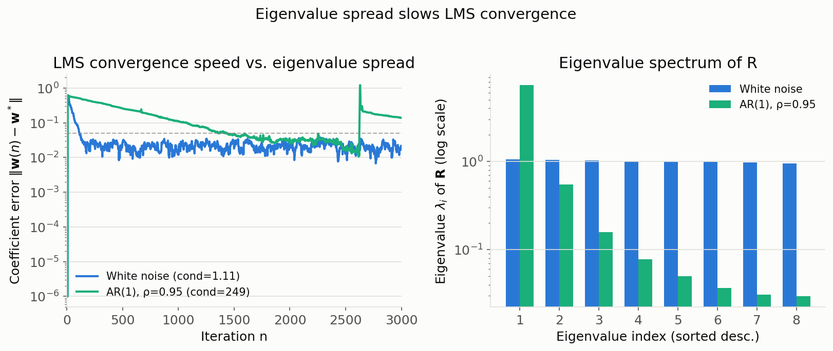
The figure visually confirms that the white-noise input (condition number near 1) decays exponentially fast, while the AR(1) input (condition number 249) decays far more slowly. The correlated-input curve also shows a transient burst of error around \(n\approx2600\) , suggesting that inputs with large eigenvalue spread also produce larger fluctuations in the instantaneous gradient.
Validating the Misadjustment Approximation
Finally, we check how closely equation (19), \(M\approx\mu\,\mathrm{tr}(\mathbf{R})/2\) , matches measured values, using \(L=8\) , white-noise input, and a \(30\) -trial Monte Carlo average.
import numpy as np

np.random.seed(3)

L = 8
N = 20000
n_trials = 30
w_true = np.array([0.5, -0.3, 0.2, 0.1, -0.05, 0.02, 0.0, 0.0])
noise_var = 0.05 ** 2  # J_min (observation noise variance)

for mu in [0.005, 0.01, 0.02, 0.04]:
    excess_list = []
    trR_list = []
    for t in range(n_trials):
        x = np.random.randn(N)
        v = 0.05 * np.random.randn(N)
        d = np.convolve(x, w_true, mode='full')[:N] + v

        w = np.zeros(L)
        e = np.zeros(N)
        for n in range(L, N):
            x_vec = x[n:n - L:-1]
            e[n] = d[n] - w @ x_vec
            w = w + mu * e[n] * x_vec

        tail = e[int(N * 0.7):]
        excess_list.append(np.mean(tail ** 2) - noise_var)

        X = np.array([x[i:i - L:-1] for i in range(L, N)])
        trR_list.append(np.trace((X.T @ X) / X.shape[0]))

    M_measured = np.mean(excess_list) / noise_var
    M_pred = mu * np.mean(trR_list) / 2
    print(f"mu={mu:.3f}: predicted M={M_pred:.4f}, measured M={M_measured:.4f}")
Results (\(J_{\min}=0.0025\) ):
mu=0.005: predicted M=0.0199, measured M=0.0189
mu=0.010: predicted M=0.0401, measured M=0.0407
mu=0.020: predicted M=0.0800, measured M=0.0864
mu=0.040: predicted M=0.1600, measured M=0.1946
Predicted and measured values agree well over \(\mu=0.005\) –\(0.02\) (roughly 5–8% error), confirming that the approximation in (19) is valid for small step sizes. At \(\mu=0.04\) the gap widens (roughly 22% error), because the derivation of (19) assumed \(\mu\lambda_i\ll1\) and dropped higher-order terms — as \(\mu\) grows, the contribution of those neglected terms becomes non-negligible.
NLMS Algorithm
Why Normalize
LMS convergence couples \(\mu\) with input power \(P_x\) (recall \(\mathrm{tr}(\mathbf{R}) \approx L P_x\) from equation (19)). With non-stationary inputs (e.g., speech), a fixed \(\mu\) is simultaneously too small in quiet periods and too large in loud ones, which compromises stability.
NLMS (Normalized LMS) normalizes the step by the input vector norm:
\[ \mathbf{w}(n+1) = \mathbf{w}(n) + \frac{\tilde{\mu}}{\lVert \mathbf{x}(n) \rVert^2 + \varepsilon}\, e(n)\, \mathbf{x}(n) \tag{20} \]The normalized step \(\tilde{\mu} \in (0, 2)\) no longer depends on input power. The small constant \(\varepsilon\) guards against division by tiny norms.
Derivation: The Minimum Disturbance Principle
Equation (20) looks arbitrary at first glance, but it can be derived from the minimum disturbance principle. The idea: move the current weight vector as little as possible while forcing the a posteriori error — the error the updated weight would produce on the same input vector \(\mathbf{x}(n)\) , \(\bar{e}(n) = d(n) - \mathbf{w}(n+1)^\top\mathbf{x}(n)\) — to exactly zero.
Restricting the update to the form \(\mathbf{w}(n+1)=\mathbf{w}(n)+\mu(n)\, e(n)\,\mathbf{x}(n)\) (fixing the gradient direction \(e(n)\mathbf{x}(n)\) and choosing only the scalar \(\mu(n)\) ) and imposing this condition gives
\[ \bar{e}(n) = d(n) - \bigl[\mathbf{w}(n) + \mu(n) e(n)\mathbf{x}(n)\bigr]^\top \mathbf{x}(n) = e(n)\bigl[1 - \mu(n)\lVert\mathbf{x}(n)\rVert^2\bigr] \tag{21} \]Setting \(\bar{e}(n)=0\) (for \(e(n)\neq 0\) ) and solving yields the unique solution
\[ \mu(n) = \frac{1}{\lVert \mathbf{x}(n) \rVert^2} \tag{22} \]Using this \(\mu(n)\) directly would cancel the current observation completely at every step, which is aggressive in practice. In practice, we add the zero-division guard \(\varepsilon\) and scale equation (22) by a factor \(\tilde\mu\in(0,2)\) , arriving back at equation (20). \(\tilde\mu=1\) corresponds exactly to the exact solution of (22) (zero a posteriori error); \(\tilde\mu<1\) is conservative (robust to observation noise), while values approaching \(\tilde\mu=2\) are more aggressive. This means LMS’s stability region \(\mu<2/\lambda_{\max}\) maps, for NLMS, onto the simple input-independent bound \(\tilde\mu<2\) .
This formulation makes clear why NLMS is robust to input-level swings. Because the step size is automatically scaled by \(1/\lVert\mathbf{x}(n)\rVert^2\) , a \(10\times\) increase in input amplitude automatically shrinks the effective step by a factor of \(1/100\) , keeping the effective update magnitude at roughly the same order at all times. Fixed-\(\mu\) LMS, by contrast, has its convergence speed and stability directly affected by changes in input amplitude — we measure this next.
LMS vs NLMS
| Feature | LMS | NLMS |
|---|---|---|
| Cost | \(O(L)\) | \(O(L)\) |
| Step bound | \(\mu < 2/(L P_x)\) (input-dependent) | \(\tilde{\mu} < 2\) (input-free) |
| Robust to input swing | Weak | Strong |
| Implementation effort | Minimal | LMS plus a normalization term |
Experiment: NLMS Robustness to Input Amplitude
As derived in equation (22), NLMS automatically adjusts its effective step size as input amplitude changes. To verify this, we compare fixed-step LMS against fixed-\(\tilde\mu\) NLMS on the same system-identification task while varying only the input amplitude.
import numpy as np

np.random.seed(2)

L = 8
N = 4000
w_true = np.array([0.5, -0.3, 0.2, 0.1, -0.05, 0.02, 0.0, 0.0])


def lms(x, d, L, mu, N):
    w = np.zeros(L)
    for n in range(L, N):
        x_vec = x[n:n - L:-1]
        e_n = d[n] - w @ x_vec
        w = w + mu * e_n * x_vec
        if not np.all(np.isfinite(w)):
            return np.full(L, np.nan)
    return w


def nlms(x, d, L, mu_tilde, N, eps=1e-6):
    w = np.zeros(L)
    for n in range(L, N):
        x_vec = x[n:n - L:-1]
        e_n = d[n] - w @ x_vec
        norm = x_vec @ x_vec + eps
        w = w + (mu_tilde / norm) * e_n * x_vec
    return w


mu_lms = 0.01        # fixed step size, tuned at scale=1
mu_tilde_nlms = 0.5   # fixed mu_tilde, tuned at scale=1

for scale in [0.1, 0.5, 1.0, 3.0, 10.0]:
    x = scale * np.random.randn(N)
    v = 0.05 * scale * np.random.randn(N)
    d = np.convolve(x, w_true, mode='full')[:N] + v

    w_l = lms(x, d, L, mu_lms, N)
    w_n = nlms(x, d, L, mu_tilde_nlms, N)

    err_l = np.linalg.norm(w_l - w_true) if np.all(np.isfinite(w_l)) else np.inf
    err_n = np.linalg.norm(w_n - w_true)
    print(f"scale={scale:>5.1f}: LMS ||w-w*||={err_l:.4e}, NLMS ||w-w*||={err_n:.4e}")
Results:
scale=  0.1: LMS ||w-w*||=4.1894e-01, NLMS ||w-w*||=1.6290e-02
scale=  0.5: LMS ||w-w*||=7.1713e-03, NLMS ||w-w*||=2.3375e-02
scale=  1.0: LMS ||w-w*||=1.1037e-02, NLMS ||w-w*||=3.0448e-02
scale=  3.0: LMS ||w-w*||=4.0226e-02, NLMS ||w-w*||=3.4492e-02
scale= 10.0: LMS ||w-w*||=inf,        NLMS ||w-w*||=2.5266e-02
Fixed-step LMS (\(\mu=0.01\)
) only performs well near scale \(1\)
. When amplitude shrinks to \(1/10\)
(scale=0.1), the effective step size becomes too small, and after \(N=4000\)
samples the coefficient error is still \(0.419\)
— far from converged. Conversely, when amplitude grows \(10\times\)
(scale=10.0), the stability limit of equation (9) is exceeded and LMS actually diverges (inf). NLMS, on the other hand, keeps \(\tilde\mu=0.5\)
fixed throughout a \(100\times\)
amplitude range (\(0.1\to10\)
), and the coefficient error stays within a tight \(0.016\)
–\(0.034\)
band — a direct experimental confirmation that the normalization term \(1/\lVert\mathbf{x}(n)\rVert^2\)
in equation (20) automatically absorbs input-power fluctuations.
Python Implementation
System Identification Example
We identify an unknown FIR system \(\mathbf{w}^\ast\) driven by white noise, using both LMS and NLMS, and plot the learning curves (squared error over iterations).
import numpy as np
import matplotlib.pyplot as plt

np.random.seed(0)

# --- Unknown system to identify ---
L = 16
w_true = np.array([0.5, -0.3, 0.2, 0.1, -0.05, 0.02,
                   0.0, 0.0, 0.0, 0.0, 0.0, 0.0,
                   0.0, 0.0, 0.0, 0.0])

# --- Input and observation ---
N = 5000
x = np.random.randn(N)
v = 0.05 * np.random.randn(N)        # measurement noise
d = np.convolve(x, w_true, mode='full')[:N] + v


def lms(x, d, L, mu):
    """Standard LMS algorithm."""
    N = len(x)
    w = np.zeros(L)
    e = np.zeros(N)
    for n in range(L, N):
        x_vec = x[n:n - L:-1]
        y = w @ x_vec
        e[n] = d[n] - y
        w = w + mu * e[n] * x_vec
    return w, e


def nlms(x, d, L, mu_tilde, eps=1e-6):
    """Normalized LMS algorithm."""
    N = len(x)
    w = np.zeros(L)
    e = np.zeros(N)
    for n in range(L, N):
        x_vec = x[n:n - L:-1]
        y = w @ x_vec
        e[n] = d[n] - y
        norm = x_vec @ x_vec + eps
        w = w + (mu_tilde / norm) * e[n] * x_vec
    return w, e


# --- Run ---
mu_lms = 0.01
mu_nlms = 0.5
w_lms, e_lms = lms(x, d, L, mu_lms)
w_nlms, e_nlms = nlms(x, d, L, mu_nlms)


# --- Learning curve (smoothed squared error) ---
def smooth(v, win=50):
    kernel = np.ones(win) / win
    return np.convolve(v ** 2, kernel, mode='same')


plt.figure(figsize=(10, 5))
plt.semilogy(smooth(e_lms), label=f'LMS (μ={mu_lms})')
plt.semilogy(smooth(e_nlms), label=f'NLMS (μ̃={mu_nlms})')
plt.xlabel('Iteration n')
plt.ylabel('Mean Squared Error')
plt.title('Learning Curves: LMS vs NLMS')
plt.legend()
plt.grid(True, alpha=0.3)
plt.tight_layout()
plt.show()

print(f"LMS   final coeff error: {np.linalg.norm(w_lms - w_true):.4f}")
print(f"NLMS  final coeff error: {np.linalg.norm(w_nlms - w_true):.4f}")
The log-scale curves show an exponential decay phase followed by a flat steady-state misadjustment floor. Increasing \(\mu\) (or \(\tilde{\mu}\) ) speeds up the initial decay but raises the floor — the canonical convergence-vs-misadjustment trade-off.
Step-Size Sensitivity
plt.figure(figsize=(10, 5))
for mu in [0.005, 0.02, 0.05, 0.1]:
    _, e = lms(x, d, L, mu)
    plt.semilogy(smooth(e), label=f'μ={mu}', alpha=0.8)
plt.xlabel('Iteration n')
plt.ylabel('Mean Squared Error')
plt.title('LMS: Sensitivity to Step Size μ')
plt.legend()
plt.grid(True, alpha=0.3)
plt.tight_layout()
plt.show()
Tiny \(\mu\) converges painfully slowly; values near the upper bound oscillate from the start. As a rule of thumb, choose at most half of the bound in (8).
Connection to the Wiener Filter
LMS converges in mean to the Wiener solution \(\mathbf{w}^\ast = \mathbf{R}^{-1}\mathbf{p}\) , with \(\mathbf{p} = E[d(n)\mathbf{x}(n)]\) :
\[ E\bigl[\mathbf{w}(n)\bigr] \xrightarrow{n \to \infty} \mathbf{w}^\ast \tag{23} \]This is exactly what we proved rigorously in equations (13)-(14). Because LMS uses an instantaneous gradient, a finite excess MSE remains (the misadjustment \(M=\mu\,\mathrm{tr}(\mathbf{R})/2\) of equation (19)). RLS (Recursive Least Squares) accelerates convergence at higher cost.
When to Use What
| Use case | Choice | Reason |
|---|---|---|
| Stationary input level | LMS | Smallest implementation, lowest cost |
| Speech / time-varying signals | NLMS | Robust to input-power swings |
| Fast convergence is critical | RLS | Quadratic cost \(O(L^2)\) but quick |
| Embedded / low-resource targets | LMS / NLMS | \(O(L)\) is sufficient |
Recent Research: Fusion with Deep Learning
Traditional LMS/NLMS/RLS filters remain the foundation of echo and noise cancellation systems, but since around 2023, hybrid architectures that combine them with deep neural networks have become increasingly common. A typical design first uses a linear adaptive filter (NLMS or a Kalman-filter-based approach) to remove the linear echo and stationary-noise components, then passes the residual through a deep neural network (DNN) to further suppress nonlinear distortion, residual echo, and non-stationary noise. Challenges such as Microsoft’s Deep Noise Suppression (DNS) Challenge and various acoustic echo cancellation challenges have driven the development of such hybrid methods.
This design is favored because the two components are complementary: the adaptive-filter stage is lightweight (\(O(L)\) ) with an explicit, theoretically grounded convergence condition and steady-state error even as input statistics change, while the DNN stage flexibly models nonlinear, non-stationary residuals that adaptive filters cannot capture. Pure end-to-end neural approaches have also been explored, but concerns around computational cost, generalization to unseen environments, and latency constraints mean they have not fully displaced adaptive filters. This area is moving quickly, so for specific method names and performance figures, consult primary sources such as each year’s challenge papers and official leaderboards.
Related Articles
- Adaptive Filter Theory and Applications in Digital Signal Processing - The theoretical starting point for this article’s LMS algorithm: derives the Wiener-Hopf equation as an MMSE problem and numerically verifies that LMS converges to the Wiener solution.
- The RLS Algorithm in Python: Recursive Least Squares and Its Equivalence to the Kalman Filter - A follow-up deriving RLS from the matrix inversion lemma, comparing its convergence speed against LMS, and demonstrating its equivalence to the Kalman filter.
- Wiener Filter: Optimal Linear Filtering Theory and Python Implementation - The optimum LMS approximates iteratively. Compares batch (frequency-domain) vs adaptive (time-domain) approaches.
- Adaptive Filters (LMS/RLS): Theory and Python Implementation - Broader treatment including RLS and noise-cancellation applications.
- Autocorrelation Function: Theory and Python Implementation - The input autocorrelation matrix \(\mathbf{R}\) governs LMS convergence speed.
- Fast Fourier Transform (FFT): Theory and Python Implementation - Foundation for frequency-domain adaptive filters (FDAF).
- Kalman Filter: Theory and Python Implementation - A different recursive estimator; RLS is mathematically equivalent to a Kalman filter.
- Moving Average Filters Compared: SMA, WMA, and EMA in Python - Contrast with fixed-coefficient filters.
- FIR and IIR Filter Comparison - Most LMS/NLMS implementations use an FIR structure; understanding FIR vs IIR clarifies step-size and convergence trade-offs.
References
- Haykin, S. (2014). Adaptive Filter Theory (5th ed.). Pearson. Chapters 5-6.
- Widrow, B., & Stearns, S. D. (1985). Adaptive Signal Processing. Prentice Hall.
- Sayed, A. H. (2008). Adaptive Filters. Wiley-IEEE Press.