Introduction
Particle Swarm Optimization (PSO) is a metaheuristic optimization technique inspired by the collective behavior of bird flocks and fish schools. Proposed by Kennedy and Eberhart in 1995, it is a gradient-free black-box optimizer that has been widely used for continuous, multimodal problems.
The defining feature of PSO is that each particle maintains a position and a velocity, and is attracted both to its own best historical position (personal best, pbest) and to the best position discovered by the entire swarm (global best, gbest). The swarm collectively converges toward promising regions of the search space much faster than pure random search.
This article reviews the PSO update rules through the lens of the inertia weight \(w\) , cognitive coefficient \(c_1\) , and social coefficient \(c_2\) , and walks through a Python implementation benchmarked on the Sphere and Rastrigin functions with convergence plots.
Algorithm
Particle State
Let the swarm size be \(N\) and the search space dimension be \(D\) . Each particle \(i \in \{1, \dots, N\}\) keeps:
- position \(\mathbf{x}_i^t \in \mathbb{R}^D\)
- velocity \(\mathbf{v}_i^t \in \mathbb{R}^D\)
- personal best \(\mathbf{p}_i^t\) (best position particle \(i\) has visited so far)
The swarm shares a single global best position \(\mathbf{g}^t = \arg\min_{i} f(\mathbf{p}_i^t)\) .
Velocity Update
The velocity of each particle is updated by:
$$ \mathbf{v}_i^{t+1} = w , \mathbf{v}_i^{t}
- c_1 \mathbf{r}_1 \odot (\mathbf{p}_i^{t} - \mathbf{x}_i^{t})
- c_2 \mathbf{r}_2 \odot (\mathbf{g}^{t} - \mathbf{x}_i^{t}) \tag{1} $$
Here \(\mathbf{r}_1, \mathbf{r}_2 \sim U[0,1]^D\) are independent uniform random vectors and \(\odot\) is the element-wise product. The three terms are:
- Term 1 \(w \, \mathbf{v}_i^t\) : inertia term, controlling how much of the previous velocity is retained
- Term 2 \(c_1 \mathbf{r}_1 \odot (\mathbf{p}_i^t - \mathbf{x}_i^t)\) : cognitive term, pulling toward the particle’s own best (pbest)
- Term 3 \(c_2 \mathbf{r}_2 \odot (\mathbf{g}^t - \mathbf{x}_i^t)\) : social term, pulling toward the swarm’s best (gbest)
Position Update
Position is advanced linearly by the new velocity:
\[ \mathbf{x}_i^{t+1} = \mathbf{x}_i^{t} + \mathbf{v}_i^{t+1} \tag{2} \]Updating pbest and gbest
After each iteration, replace the personal best whenever the current position improves the objective:
\[ \mathbf{p}_i^{t+1} = \begin{cases} \mathbf{x}_i^{t+1} & \text{if } f(\mathbf{x}_i^{t+1}) < f(\mathbf{p}_i^{t}) \\ \mathbf{p}_i^{t} & \text{otherwise} \end{cases} \tag{3} \]The global best is then refreshed:
\[ \mathbf{g}^{t+1} = \arg\min_{i} f(\mathbf{p}_i^{t+1}) \tag{4} \]Hyperparameters
Inertia Weight \(w\)
\(w\) governs the trade-off between exploration and exploitation.
- Large \(w\) (e.g. \(w \approx 0.9\) ): particles strongly retain previous velocity, encouraging wide-area search
- Small \(w\) (e.g. \(w \approx 0.4\) ): velocity decays quickly, promoting fine-grained local refinement
In practice, linearly decreasing inertia weight (LDIW) is the de facto standard, exploring broadly early on and converging late:
\[ w_t = w_{\max} - (w_{\max} - w_{\min}) \cdot \frac{t}{T_{\max}} \tag{5} \]Typical values are \(w_{\max} = 0.9\) and \(w_{\min} = 0.4\) .
Cognitive Coefficient \(c_1\) and Social Coefficient \(c_2\)
\(c_1\) and \(c_2\) weight the pull toward the particle’s own experience and the swarm’s experience, respectively.
- \(c_1 \gg c_2\) : particles favor their own history, leading to more independent search
- \(c_1 \ll c_2\) : pull toward the global best dominates, often causing premature convergence
Clerc & Kennedy (2002) derived a constriction coefficient form yielding \(w = 0.7298\) and \(c_1 = c_2 = 2.05\) . A widely used default is \(w = 0.729, c_1 = c_2 = 1.4944\) .
Velocity Clipping
To prevent particles from diverging out of the search domain, each velocity component is typically clipped to \(|v_{i,d}| \leq v_{\max}\) , where \(v_{\max}\) is around 10–20% of the search range width.
Benchmark Functions
Sphere Function (Unimodal)
\[ f_{\text{sphere}}(\mathbf{x}) = \sum_{i=1}^{D} x_i^2 \tag{6} \]The global minimum is \(f(\mathbf{0}) = 0\) . Being unimodal, PSO converges easily.
Rastrigin Function (Multimodal)
\[ f_{\text{rastrigin}}(\mathbf{x}) = 10 D + \sum_{i=1}^{D} \left[ x_i^2 - 10 \cos(2\pi x_i) \right] \tag{7} \]The global minimum is again \(f(\mathbf{0}) = 0\) , but the landscape has many local minima. With the wrong inertia weight or coefficients, the swarm may stagnate at a local minimum.
Python Implementation
A minimal NumPy-only PSO with linearly decreasing inertia weight and velocity clipping:
import numpy as np
import matplotlib.pyplot as plt


def sphere(x):
    """Sphere function (unimodal)"""
    return np.sum(x**2, axis=-1)


def rastrigin(x):
    """Rastrigin function (multimodal)"""
    return 10 * x.shape[-1] + np.sum(x**2 - 10 * np.cos(2 * np.pi * x), axis=-1)


class PSO:
    def __init__(self, dim, n_particles=40, bounds=(-5.12, 5.12),
                 w_max=0.9, w_min=0.4, c1=1.4944, c2=1.4944,
                 v_max_ratio=0.2):
        self.dim = dim
        self.n_particles = n_particles
        self.bounds = bounds
        self.w_max = w_max
        self.w_min = w_min
        self.c1 = c1
        self.c2 = c2
        # v_max is a fraction of the search range width
        self.v_max = v_max_ratio * (bounds[1] - bounds[0])

    def initialize(self):
        low, high = self.bounds
        x = np.random.uniform(low, high, (self.n_particles, self.dim))
        v = np.random.uniform(-self.v_max, self.v_max,
                              (self.n_particles, self.dim))
        return x, v

    def run(self, objective, max_iter=200):
        x, v = self.initialize()
        f = objective(x)

        # Initialize pbest / gbest
        pbest = x.copy()
        pbest_f = f.copy()
        g_idx = int(np.argmin(pbest_f))
        gbest = pbest[g_idx].copy()
        gbest_f = float(pbest_f[g_idx])

        history = [gbest_f]

        for t in range(max_iter):
            # Linearly decreasing inertia weight
            w = self.w_max - (self.w_max - self.w_min) * (t / max_iter)

            # Velocity update (Eq. 1)
            r1 = np.random.random((self.n_particles, self.dim))
            r2 = np.random.random((self.n_particles, self.dim))
            v = (w * v
                 + self.c1 * r1 * (pbest - x)
                 + self.c2 * r2 * (gbest - x))
            v = np.clip(v, -self.v_max, self.v_max)

            # Position update (Eq. 2)
            x = x + v
            x = np.clip(x, *self.bounds)

            # Evaluate and update pbest / gbest
            f = objective(x)
            improved = f < pbest_f
            pbest[improved] = x[improved]
            pbest_f[improved] = f[improved]

            g_idx = int(np.argmin(pbest_f))
            if pbest_f[g_idx] < gbest_f:
                gbest = pbest[g_idx].copy()
                gbest_f = float(pbest_f[g_idx])

            history.append(gbest_f)

        return gbest, gbest_f, history


# --- Run ---
np.random.seed(42)
pso_sphere = PSO(dim=10)
_, best_sphere, hist_sphere = pso_sphere.run(sphere, max_iter=200)

np.random.seed(42)
pso_rastrigin = PSO(dim=10)
_, best_rastrigin, hist_rastrigin = pso_rastrigin.run(rastrigin, max_iter=200)

print(f"Sphere    best fitness: {best_sphere:.6e}")
print(f"Rastrigin best fitness: {best_rastrigin:.6e}")

# --- Convergence plot ---
plt.figure(figsize=(10, 5))
plt.plot(hist_sphere, label='Sphere (10D)')
plt.plot(hist_rastrigin, label='Rastrigin (10D)')
plt.xlabel('Iteration')
plt.ylabel('Best Objective Value')
plt.title('PSO Convergence on Sphere and Rastrigin')
plt.yscale('log')
plt.grid(True, alpha=0.3)
plt.legend()
plt.tight_layout()
plt.show()
Running the code above (seed=42, 10 dimensions, 40 particles, 200 iterations) gives:
Sphere    best fitness: 2.547928e-15
Rastrigin best fitness: 6.964713e+00
Being unimodal, Sphere converges to roughly \(10^{-15}\) , while Rastrigin’s multimodal landscape leaves the swarm stuck near \(7\) , far from the global minimum \(0\) . How strongly the inertia schedule, swarm size, and coefficients matter is quantified in the next sections.
Effect of Inertia Weight on Convergence
Comparing different fixed \(w\) values is straightforward:
import numpy as np
import matplotlib.pyplot as plt

results = {}
for w in [0.3, 0.5, 0.7, 0.9]:
    np.random.seed(0)
    pso = PSO(dim=10, w_max=w, w_min=w)  # fixed inertia weight
    _, _, history = pso.run(rastrigin, max_iter=200)
    results[w] = history

plt.figure(figsize=(10, 5))
for w, history in results.items():
    plt.plot(history, label=f'w = {w}')
plt.xlabel('Iteration')
plt.ylabel('Best Objective Value')
plt.title('Effect of Inertia Weight on Rastrigin (10D)')
plt.yscale('log')
plt.grid(True, alpha=0.3)
plt.legend()
plt.tight_layout()
plt.show()
Running with the same seed=0, the final best fitness after 200 iterations was:
| \(w\) (fixed) | Final best fitness |
|---|---|
| 0.3 | 3.981448 |
| 0.5 | 15.919330 |
| 0.7 | 4.974795 |
| 0.9 | 35.174607 |
\(w = 0.9\) performed worst because velocity barely decays and local refinement never really kicks in; \(w = 0.5\) also lands in an awkward middle ground between exploration and exploitation. \(w = 0.3\) and \(w = 0.7\) look relatively good here, but this is a single-seed result and the relationship between \(w\) and final fitness is not monotonic (as the next section shows, a fixed \(w\) trades off “stagnating after losing diversity too early” against “converging too slowly,” and this trade-off is highly seed-dependent — a time-varying schedule like LDIW is more robust).
Convergence and Divergence: A Stability Analysis
The previous section swept fixed values of \(w\) experimentally. But which parameter region actually guarantees convergence of the velocity/position update (Eqs. 1, 2), and where does it start to diverge? Here we follow the standard stability analysis of van den Bergh (2001), Clerc & Kennedy (2002), and Trelea (2003) to derive the boundary, then confirm it numerically.
Derivation via a simplified model
For a tractable analysis we make the following standard simplifications.
- Focus on a single particle in one dimension (each dimension and particle behaves independently in the update equations, so this loses no generality)
- Assume the personal best \(\mathbf{p}_i\) and global best \(\mathbf{g}\) have collapsed onto the same point \(p\) (a local stability analysis around a stagnation point)
- Replace the random draws \(r_1, r_2 \sim U[0,1]\) with their expectation \(E[r_1] = E[r_2] = 0.5\) (a deterministic approximation)
Defining the deviation \(e_t = x_t - p\) , the second and third terms of Eq. (1) collapse to \(c_1 r_1 (p - x_t) + c_2 r_2 (p - x_t) \to -\phi\, e_t\) (with \(\phi = (c_1+c_2)/2\) ), so the update rule becomes
\[ v_{t+1} = w\, v_t - \phi\, e_t \] \[ e_{t+1} = e_t + v_{t+1} = w\, v_t + (1-\phi)\, e_t \]In matrix form,
$$ \begin{pmatrix} v_{t+1} \ e_{t+1} \end{pmatrix}
\begin{pmatrix} w & -\phi \ w & 1-\phi \end{pmatrix} \begin{pmatrix} v_t \ e_t \end{pmatrix} \tag{8} $$
Eigenvalues and the stability condition
This linear recurrence converges to \(e_t \to 0\) as \(t \to \infty\) if and only if every eigenvalue \(\lambda\) of the coefficient matrix lies inside the unit circle (\(|\lambda| < 1\) ). With trace \(w+1-\phi\) and determinant \(w\) , the characteristic equation is
\[ \lambda^2 - (1 + w - \phi)\lambda + w = 0 \tag{9} \]For a quadratic \(\lambda^2 - b_1 \lambda + b_0 = 0\) , the Jury stability criterion places both roots inside the unit circle iff \(|b_0| < 1\) , \(1 - b_1 + b_0 > 0\) , and \(1 + b_1 + b_0 > 0\) . Substituting \(b_1 = 1+w-\phi\) and \(b_0 = w\) from Eq. (9):
- \(|w| < 1\)
- \(1-(1+w-\phi)+w = \phi > 0\)
- \(1+(1+w-\phi)+w = 2+2w-\phi > 0 \iff \phi < 2(1+w)\)
Converting \(\phi = (c_1+c_2)/2\) back gives the stability condition:
\[ w < 1, \qquad 0 < c_1 + c_2 < 4(1+w) \]This exact inequality (Eqs. 16.38–16.39) is also presented in Engelbrecht’s (2007) textbook Computational Intelligence: An Introduction, Chapter 16, summarizing van den Bergh’s convergence analysis. Clerc & Kennedy’s (2002) constriction coefficients \(w=0.7298, c_1=c_2=2.05\) (\(c_1+c_2=4.10\) , bound \(4(1+w)=6.92\) ) and this article’s default \(w=0.729, c_1=c_2=1.4944\) (\(c_1+c_2 \approx 2.99\) ) both sit comfortably inside this stability region.
Numerical experiment: divergence near and beyond the boundary
We implement the simplified model (Eq. 8) directly and track the deviation \(|e_t|\) starting from \(e_0=1\) .
import numpy as np


def simulate_deviation(w, c1, c2, T=150, seed=0, e0=1.0):
    """Track the deviation e_t = x_t - p of the simplified model (Eq. 8),
    corresponding to the setting pbest = gbest = p used in the local stability analysis."""
    rng = np.random.default_rng(seed)
    v, e = 0.0, e0
    traj = [abs(e)]
    for _ in range(T):
        r1, r2 = rng.random(), rng.random()
        v = w * v - (c1 * r1 + c2 * r2) * e
        e = e + v
        traj.append(abs(e) + 1e-300)
    return np.array(traj)


configs = [
    ("Clerc-Kennedy (w=0.7298, c1=c2=1.4962)", 0.7298, 1.4962, 1.4962),
    ("w=0.70, c1=c2=3.0 (inside bound)", 0.70, 3.0, 3.0),
    ("w=0.70, c1=c2=4.0 (exceeds bound)", 0.70, 4.0, 4.0),
]

for label, w, c1, c2 in configs:
    bound = 4 * (1 + w)
    finals = [simulate_deviation(w, c1, c2, T=150, seed=s)[-1] for s in range(50)]
    print(f"{label:42} c1+c2={c1+c2:.2f} bound={bound:.2f} "
          f"median|e_150|={np.median(finals):.3e}")
The results (median over 50 seeds) are:
Clerc-Kennedy (w=0.7298, c1=c2=1.4962) c1+c2=2.99 bound=6.92 median|e_150|=2.374e-07
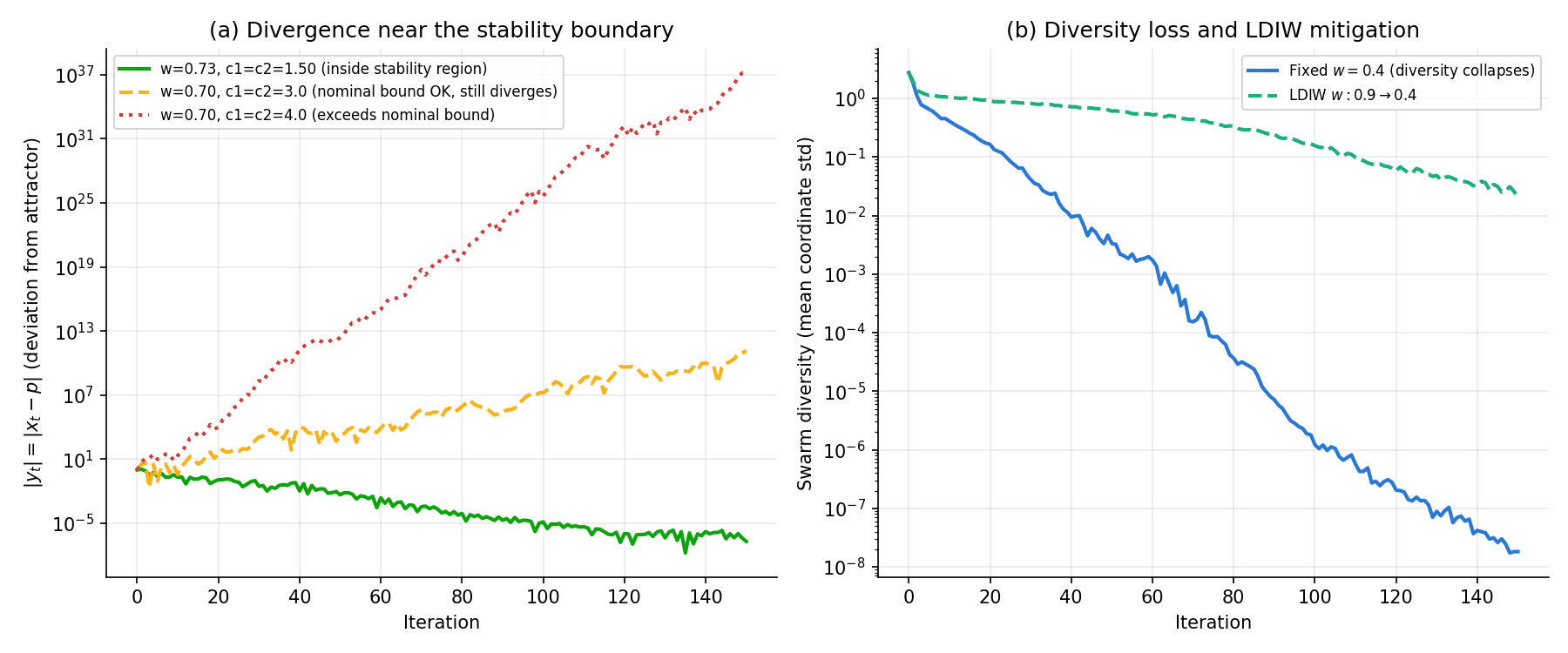
w=0.70, c1=c2=3.0 (inside bound) c1+c2=6.00 bound=6.80 median|e_150|=1.047e+12
w=0.70, c1=c2=4.0 (exceeds bound) c1+c2=8.00 bound=6.80 median|e_150|=2.010e+35
The Clerc-Kennedy coefficients converge smoothly to about \(10^{-7}\) , while \(c_1=c_2=3.0\) (\(w=0.7\) ) satisfies the boundary \(4(1+w)=6.8\) from Eq. (9) yet still diverges to a median of \(10^{12}\) across 50 seeds. \(c_1=c_2=4.0\) diverges even more violently, to \(10^{35}\) .
This happens because Eq. (9)’s analysis is only a deterministic (expected-value) approximation that replaces the random draws \(r_1, r_2\) with their expectation \(0.5\) . The actual PSO recursion redraws random numbers at every step, and as Jiang, Luo & Yang (2007) and Poli (2009) point out, the expected-value trajectory can converge while the variance of the trajectory still diverges (Cleghorn & Engelbrecht frame this as the distinction between “order-1 stability” and “order-2 stability”). In other words, \(0 < c_1+c_2 < 4(1+w)\) is only a necessary-condition heuristic and can be insufficient to prevent stochastic divergence. In practice, it is safer to choose \(c_1+c_2\) well below the boundary — as Clerc-Kennedy and this article’s defaults do — or to combine it with velocity clipping.
Panel (a) below visualizes \(|e_t|\) over time for these three configurations, from a single seed.
Diversity Loss and Premature Convergence
Separately from the stability analysis above, PSO carries a risk of premature convergence, in which every particle collapses onto the same local optimum (near gbest) and the search effectively stops. The social term \(c_2 r_2 (\mathbf{g}^t - \mathbf{x}_i^t)\) in Eq. (1) pulls all particles toward the same point, and when the inertia term \(w \mathbf{v}_i^t\) is small, velocity decays quickly, so inter-particle distance (diversity) collapses fast. Once diversity is gone, the cognitive and social terms themselves have almost nothing left to drive, and the swarm can no longer explore new regions.
Numerical experiment: diversity collapse and LDIW mitigation
We use a small swarm (\(N=10\) ) on the 10-dimensional Rastrigin function and compare (a) a fixed inertia weight \(w=0.4\) against (b) linearly decreasing inertia weight (LDIW, \(w: 0.9 \to 0.4\) ). As a diversity metric we track \(\bar{\sigma}_t = \frac{1}{D}\sum_{d=1}^{D} \mathrm{std}(x_{1,d}^t, \dots, x_{N,d}^t)\) , the per-dimension coordinate standard deviation averaged over dimensions.
import numpy as np


def rastrigin(x):
    return 10 * x.shape[-1] + np.sum(x**2 - 10 * np.cos(2 * np.pi * x), axis=-1)


def run_pso_track_diversity(dim, n_particles, w_max, w_min, decay, c1, c2,
                             max_iter=150, bounds=(-5.12, 5.12), v_max_ratio=0.2, seed=0):
    rng = np.random.default_rng(seed)
    low, high = bounds
    v_max = v_max_ratio * (high - low)
    x = rng.uniform(low, high, (n_particles, dim))
    v = rng.uniform(-v_max, v_max, (n_particles, dim))
    f = rastrigin(x)
    pbest, pbest_f = x.copy(), f.copy()
    g_idx = int(np.argmin(pbest_f))
    gbest_f = float(pbest_f[g_idx])
    diversity = [float(np.mean(np.std(x, axis=0)))]
    for t in range(max_iter):
        w = w_max - (w_max - w_min) * (t / max_iter) if decay else w_max
        r1 = rng.random((n_particles, dim))
        r2 = rng.random((n_particles, dim))
        v = w * v + c1 * r1 * (pbest - x) + c2 * r2 * (pbest[g_idx] - x)
        v = np.clip(v, -v_max, v_max)
        x = np.clip(x + v, low, high)
        f = rastrigin(x)
        improved = f < pbest_f
        pbest[improved], pbest_f[improved] = x[improved], f[improved]
        g_idx = int(np.argmin(pbest_f))
        gbest_f = min(gbest_f, float(pbest_f[g_idx]))
        diversity.append(float(np.mean(np.std(x, axis=0))))
    return gbest_f, diversity


N_SEEDS = 30
for label, w_max, decay in [("fixed w=0.4", 0.4, False), ("LDIW w:0.9->0.4", 0.9, True)]:
    finals, collapse_iters = [], []
    for seed in range(N_SEEDS):
        best_f, diversity = run_pso_track_diversity(
            dim=10, n_particles=10, w_max=w_max, w_min=0.4, decay=decay,
            c1=1.4944, c2=1.4944, max_iter=150, seed=seed)
        finals.append(best_f)
        threshold = 0.01 * diversity[0]
        collapse_iters.append(next((i for i, d in enumerate(diversity) if d < threshold), len(diversity)))
    print(f"{label:16} collapse_iter(mean)={np.mean(collapse_iters):.1f}  "
          f"final_f(mean±std)={np.mean(finals):.2f}±{np.std(finals):.2f}")
The results are:
fixed w=0.4      collapse_iter(mean)=30.6  final_f(mean±std)=20.77±10.64
LDIW w:0.9->0.4  collapse_iter(mean)=120.1  final_f(mean±std)=16.66±6.81
Averaged over 30 seeds (\(N=10\)
, \(c_1=c_2=1.4944\)
, max_iter=150, Rastrigin 10D):
| Setting | Mean iterations until diversity < 1% of initial | Final best fitness (mean ± std) |
|---|---|---|
| Fixed \(w=0.4\) (no decay) | 30.6 | \(20.77 \pm 10.64\) |
| LDIW (\(w: 0.9\to 0.4\) ) | 120.1 | \(16.66 \pm 6.81\) |
With a fixed \(w=0.4\) , diversity collapses to under 1% of its initial value after only about 30 iterations on average, after which the swarm sits clustered near a local optimum and stagnates. LDIW delays this collapse to an average of 120 iterations, roughly quadrupling the effective search budget, which also improves both the mean and variance of the final fitness (though LDIW does not avoid eventual diversity loss altogether — it only buys more time before the collapse).
Panel (b) of the figure above (shared with the previous section) shows the diversity trajectory \(\bar{\sigma}_t\) averaged over the 30 seeds for both settings. The fixed \(w=0.4\) curve falls off exponentially fast, while LDIW retains high diversity early on thanks to its larger initial \(w\) , converging more gradually toward the end.
Beyond the LDIW schedule used here, other mitigations for diversity loss include randomly re-initializing particle velocities and two-swarm cooperative PSO (TCPSO), which splits the swarm into an exploration group and an exploitation group. TCPSO’s mechanism, the derivation of its convergence conditions, and practical countermeasures against local optima are covered in detail in The Mathematics of Two-Swarm Cooperative PSO (TCPSO) .
Comparison with Other Optimizers
| Method | Population-based | Main mechanism | Multimodality | Expensive evaluations |
|---|---|---|---|---|
| PSO | Yes | Velocity / position update with pbest, gbest | Medium | Poor fit |
| GA | Yes | Selection / crossover / mutation | High | Poor fit |
| CEM | Yes | Iterative distribution update | Medium | Poor fit |
| SA | No | Metropolis acceptance with temperature | High | Poor fit |
| Bayesian Opt | No | Gaussian process surrogate | Medium | Excellent |
PSO has very few hyperparameters and a simple implementation, making it practical for medium-dimensional continuous problems. When evaluations are extremely expensive (e.g. real-world experiments), Bayesian optimization that minimizes evaluation count is usually more appropriate.
Benchmark: matching evaluation budgets against GA and SA
Genetic Algorithms: Fundamentals and Python Implementation
and
Simulated Annealing: Theory and Python Implementation
each benchmark on the 10-dimensional Rastrigin function independently, but GA uses pop_size=200, max_generations=300 (60,000 evaluations) while SA uses max_iter=10000 (10,000 evaluations) — the conditions differ too much for a direct comparison. Here we equalize the evaluation budget to about 8000 for all three (PSO: 40 particles × 200 iterations, GA: population 40 × 200 generations, SA: 8000 iterations) and run 10 seeds each on the Sphere and Rastrigin functions (both 10-dimensional).
import numpy as np


def sphere(x):
    return np.sum(x**2, axis=-1)


def rastrigin(x):
    return 10 * x.shape[-1] + np.sum(x**2 - 10 * np.cos(2 * np.pi * x), axis=-1)


def run_pso(objective, dim, n_particles=40, max_iter=200, bounds=(-5.12, 5.12),
            w_max=0.9, w_min=0.4, c1=1.4944, c2=1.4944, v_max_ratio=0.2, seed=0):
    rng = np.random.default_rng(seed)
    low, high = bounds
    v_max = v_max_ratio * (high - low)
    x = rng.uniform(low, high, (n_particles, dim))
    v = rng.uniform(-v_max, v_max, (n_particles, dim))
    f = objective(x)
    pbest, pbest_f = x.copy(), f.copy()
    g_idx = int(np.argmin(pbest_f))
    gbest_f = float(pbest_f[g_idx])
    for t in range(max_iter):
        w = w_max - (w_max - w_min) * (t / max_iter)
        r1 = rng.random((n_particles, dim))
        r2 = rng.random((n_particles, dim))
        v = w * v + c1 * r1 * (pbest - x) + c2 * r2 * (pbest[g_idx] - x)
        v = np.clip(v, -v_max, v_max)
        x = np.clip(x + v, low, high)
        f = objective(x)
        improved = f < pbest_f
        pbest[improved], pbest_f[improved] = x[improved], f[improved]
        g_idx = int(np.argmin(pbest_f))
        gbest_f = min(gbest_f, float(pbest_f[g_idx]))
    return gbest_f


def run_ga(objective, dim, pop_size=40, max_generations=200, bounds=(-5.12, 5.12), seed=0):
    rng = np.random.default_rng(seed)
    low, high = bounds

    def tournament(population, fitness, k=3):
        idx = rng.integers(0, pop_size, k)
        return population[idx[np.argmin(fitness[idx])]]

    def crossover(p1, p2, alpha=0.5):
        lo = np.minimum(p1, p2) - alpha * np.abs(p1 - p2)
        hi = np.maximum(p1, p2) + alpha * np.abs(p1 - p2)
        return np.clip(rng.uniform(lo, hi), low, high)

    def mutate(ind, sigma=0.1, rate=0.1):
        mask = rng.random(dim) < rate
        ind = ind.copy()
        ind[mask] += rng.normal(0, sigma * (high - low), size=mask.sum())
        return np.clip(ind, low, high)

    population = rng.uniform(low, high, (pop_size, dim))
    best_f = float(np.min(objective(population)))
    for _ in range(max_generations):
        fitness = objective(population)
        best_idx = int(np.argmin(fitness))
        best_f = min(best_f, float(fitness[best_idx]))
        new_pop = [population[best_idx].copy()]  # elitism
        while len(new_pop) < pop_size:
            child = mutate(crossover(tournament(population, fitness), tournament(population, fitness)))
            new_pop.append(child)
        population = np.array(new_pop[:pop_size])
    return min(best_f, float(np.min(objective(population))))


def run_sa(objective, dim, bounds=(-5.12, 5.12), T_init=100.0, alpha=0.995, max_iter=7999, seed=0):
    rng = np.random.default_rng(seed)
    low, high = bounds
    x = rng.uniform(low, high, size=dim)
    f = float(objective(x[None, :])[0])
    best_f, T = f, T_init
    for _ in range(max_iter):
        x_new = np.clip(x + rng.normal(0, 1.0, size=dim), low, high)
        f_new = float(objective(x_new[None, :])[0])
        if f_new < f or rng.random() < np.exp(-(f_new - f) / T):
            x, f = x_new, f_new
            best_f = min(best_f, f)
        T *= alpha
    return best_f


N_SEEDS = 10
for fname, fn in [("Sphere", sphere), ("Rastrigin", rastrigin)]:
    print(f"=== {fname} ===")
    for label, runner in [
        ("PSO", lambda seed: run_pso(fn, dim=10, seed=seed)),
        ("GA", lambda seed: run_ga(fn, dim=10, seed=seed)),
        ("SA", lambda seed: run_sa(fn, dim=10, seed=seed)),
    ]:
        finals = np.array([runner(seed) for seed in range(N_SEEDS)])
        print(f"  {label}: mean={np.mean(finals):.4e}  median={np.median(finals):.4e}")
The results are:
=== Sphere ===
  PSO: mean=1.9328e-15  median=1.2058e-15
  GA:  mean=4.0921e-03  median=3.8573e-03
  SA:  mean=9.4169e-01  median=9.7838e-01
=== Rastrigin ===
  PSO: mean=6.8654e+00  median=5.9704e+00
  GA:  mean=7.2726e+00  median=6.9409e+00
  SA:  mean=4.6989e+01  median=4.4726e+01
Over 10 seeds, at a matched evaluation budget of about 8000:
| Method | Sphere (mean) | Sphere (median) | Rastrigin (mean) | Rastrigin (median) |
|---|---|---|---|---|
| PSO | \(1.93 \times 10^{-15}\) | \(1.21 \times 10^{-15}\) | \(6.87\) | \(5.97\) |
| GA | \(4.09 \times 10^{-3}\) | \(3.86 \times 10^{-3}\) | \(7.27\) | \(6.94\) |
| SA | \(9.42 \times 10^{-1}\) | \(9.78 \times 10^{-1}\) | \(46.99\) | \(44.73\) |
On the unimodal Sphere function, PSO reaches values about 12 orders of magnitude smaller than GA and nearly 15 orders smaller than SA, reflecting how smoothly it descends a single-basin landscape without gradient information. On the multimodal Rastrigin function, PSO and GA are roughly tied (mean \(6.87\) vs. \(7.27\) ), while the single-solution SA (which, with this neighborhood width and cooling schedule, struggles to escape local optima) trails well behind at a mean of \(46.99\) . This matches the commonly stated rule of thumb: PSO tends to win on unimodal continuous optimization, while PSO and GA run neck-and-neck on multimodal landscapes.
Recent Research Trends (2023 and Later)
Although PSO is a classical method dating back to 1995, research extending and applying it has continued actively since 2023.
- Prompt optimization for LLMs: Hsieh et al. (2025, Expert Systems) combine PSO with large language models (LLMs) to search a continuous prompt-embedding space. Conversely, Shinohara et al. (2025, arXiv:2504.09247), “Large Language Models as Particle Swarm Optimizers,” have the LLM itself imitate PSO’s update rule — showing that PSO’s “particle-based iterative update” skeleton is still being referenced in the LLM era.
- Hyperparameter search: Hameed et al. (2025, arXiv:2504.14126), “Large Language Model Enhanced Particle Swarm Optimization for Hyperparameter Tuning for Deep Learning Models,” use an LLM to assist PSO’s candidate generation, reducing the number of evaluations needed for hyperparameter search in deep learning models.
- Multi-objective PSO (MOPSO): MOPSO, which optimizes several objectives simultaneously, is organized into Pareto-dominance-based, decomposition-based, and indicator-based families, and surveys such as the 2024 “Survey of multi-objective particle swarm optimization algorithms and their applications” (Journal of Zhejiang University) continue to appear.
- Quantum-behaved PSO (QPSO): QPSO, which borrows ideas from quantum mechanics, remains an active variant aimed at mitigating premature convergence on multimodal problems; a 2025 Scientific Reports paper reports an application of quantum-inspired PSO to feature-selection tasks.
Each of these lines of work tackles, from a different angle, the same core PSO challenges surveyed in this article: the balance between convergence and divergence, and the loss of diversity.
Summary
- PSO is built from velocity/position updates (Eqs. 1, 2) and pbest/gbest updates (Eqs. 3, 4)
- Inertia weight \(w\) , cognitive coefficient \(c_1\) , and social coefficient \(c_2\) weight diversity, self-experience, and swarm-experience respectively
- Linearly decreasing inertia weight (Eq. 5) and velocity clipping are practically essential for multimodal problems like Rastrigin
- Convergence is fast on Sphere; on Rastrigin the configuration largely determines the outcome
- The deterministic approximation gives \(w<1,\ 0<c_1+c_2<4(1+w)\) as a convergence guideline (Eqs. 8, 9), but the actual stochastic PSO can still diverge even inside this bound
- With a small, fixed inertia weight, diversity can collapse within a few dozen iterations, causing premature convergence; LDIW is an effective mitigation that delays this collapse
- At a matched evaluation budget, PSO substantially outperforms GA and SA on the unimodal Sphere function, while PSO and GA are roughly tied on the multimodal Rastrigin function
Reading this together with the rest of the optimization series clarifies which method fits which problem class.
Related Articles
- Genetic Algorithms: Fundamentals and Python Implementation - Evolutionary metaheuristic. PSO moves continuously via velocity, while GA evolves discretely via crossover and mutation.
- Simulated Annealing: Theory and Python Implementation - Comparing PSO with the single-solution SA highlights the characteristics of population-based methods.
- Cross-Entropy Method: A Practical Monte Carlo Optimization Technique - CEM iteratively updates a probability distribution; the pull of all particles toward gbest in PSO has a similar flavor.
- Bayesian Optimization: Fundamentals and Python Implementation - Designed for expensive-evaluation settings. The problem regimes targeted by PSO and Bayesian optimization differ substantially.
- Monte Carlo Optimization Methods Comparison (CEM/SA/GA/MPPI/PSO) - Hub article comparing five Monte Carlo optimizers including PSO under a common sample/evaluate/update skeleton, positioning PSO’s inertia/social-coefficient dynamics against the other methods.
- The Mathematics of Two-Swarm Cooperative PSO (TCPSO) - Addresses the diversity-loss and premature-convergence problem covered in this article by coordinating two swarms with distinct exploration and exploitation roles, including a derivation of their convergence conditions.
References
- Kennedy, J., & Eberhart, R. (1995). “Particle Swarm Optimization”. Proceedings of IEEE International Conference on Neural Networks, 4, 1942-1948.
- Shi, Y., & Eberhart, R. (1998). “A modified particle swarm optimizer”. Proceedings of IEEE International Conference on Evolutionary Computation, 69-73.
- Clerc, M., & Kennedy, J. (2002). “The particle swarm – explosion, stability, and convergence in a multidimensional complex space”. IEEE Transactions on Evolutionary Computation, 6(1), 58-73.
- van den Bergh, F. (2001). “An Analysis of Particle Swarm Optimizers”. PhD thesis, University of Pretoria.
- Trelea, I. C. (2003). “The particle swarm optimization algorithm: convergence analysis and parameter selection”. Information Processing Letters, 85(6), 317-325.
- Engelbrecht, A. P. (2007). Computational Intelligence: An Introduction (2nd ed.), Chapter 16. Wiley.
- Jiang, M., Luo, Y. P., & Yang, S. Y. (2007). “Stochastic convergence analysis and parameter selection of the standard particle swarm optimization algorithm”. Information Processing Letters, 102(1), 8-16.
- Poli, R. (2009). “Mean and variance of the sampling distribution of particle swarm optimizers during stagnation”. IEEE Transactions on Evolutionary Computation, 13(4), 712-721.
- Cleghorn, C. W., & Engelbrecht, A. P. (2014). “A generalized theoretical deterministic particle swarm model”. Swarm Intelligence, 8(1), 35-59.
- Hsieh et al. (2025). “A Particle Swarm Optimization-Based Approach Coupled With Large Language Models for Prompt Optimization”. Expert Systems. Wiley.
- Shinohara, Y., Xu, J., Li, T., & Iba, H. (2025). “Large Language Models as Particle Swarm Optimizers”. arXiv:2504.09247.
- Hameed, S., Qolomany, B., Belhaouari, S. B., Abdallah, M., Qadir, J., & Al-Fuqaha, A. (2025). “Large Language Model Enhanced Particle Swarm Optimization for Hyperparameter Tuning for Deep Learning Models”. arXiv:2504.14126.