Convolution and Correlation Fundamentals: Theory, Convolution Theorem, and Python Implementation

Introduction

Convolution and correlation are foundational operations in signal processing. They underpin filtering, feature extraction, pattern matching, and system identification, and they form the mathematical bedrock of frequency-domain methods such as the FFT and the wavelet transform .

This article reviews the continuous and discrete definitions of convolution and correlation, clarifies how the two are related, and uses the convolution theorem to bridge the time and frequency domains. We then implement and benchmark np.convolve, scipy.signal.correlate, and FFT-based fast convolution in Python. Finally, we show that the moving average filter is simply a convolution with a box window.

Definition of Convolution

Continuous Convolution

For two continuous functions \(f(t)\) and \(g(t)\) , convolution is defined as

Intuitively, we flip \(g\) in time, slide it by \(t\) , multiply with \(f\) , and integrate. Because the response of a linear time-invariant (LTI) system is the convolution of its input with its impulse response, filtering is convolution in the most fundamental sense.

Discrete Convolution

For discrete signals \(x[n]\) and \(h[n]\) ,

In practice, we time-reverse \(h\) , slide it across \(x\) , take elementwise products, and sum. If \(x\) has length \(N\) and \(h\) has length \(M\) , the linear convolution output has length \(N + M - 1\) .

Algebraic Properties

Convolution satisfies several useful identities.

• Commutativity: \(x * h = h * x\)
• Associativity: \((x * h) * g = x * (h * g)\)
• Distributivity: \(x * (h + g) = x * h + x * g\)

Cascaded filters can therefore be merged into a single equivalent kernel.

Definition of Correlation

Cross-Correlation

The cross-correlation of \(x[n]\) and \(y[n]\) at lag \(\ell\) is

It measures how similar \(x\) is to a shifted version of \(y\) , and is widely used for delay estimation and template matching.

Auto-Correlation

When \(y = x\) , we obtain the auto-correlation, which detects periodicities and self-similarity in a single signal:

\(R_{xx}[0]\) equals the total energy (or variance) and is the global maximum of \(R_{xx}\) .

Relationship to Convolution

Cross-correlation and convolution differ only in whether the second argument is time-reversed. For real signals,

so correlation can be implemented as convolution with a time-reversed kernel. For complex signals, also take the complex conjugate (\(\tilde{y}[n] = y^*[-n]\) ).

Relationship to the Matched Filter

Why does correlation turn out to be the operation performed by a “matched filter”? We derive this as an optimal-detection problem under noise. Suppose a known waveform (template) \(s[n]\) (\(n = 0, \dots, K-1\) ) is received buried in additive white noise \(w[n]\) (zero mean, variance \(\sigma^2\) , independent samples):

Pass \(r[n]\) through a length-\(K\) FIR filter \(h[n]\) , producing \(y[n] = (r * h)[n]\) . Focus on the instant \(n = K-1\) , when the template exactly fills the filter window:

The signal term \(S\) is a deterministic constant, while the noise term \(W\) is a random variable with variance \(\text{Var}[W] = \sigma^2 \sum_{k=0}^{K-1} h[K-1-k]^2\) (variance adds linearly because the \(w[k]\) are independent). The output SNR is

Applying the Cauchy–Schwarz inequality to the numerator,

with equality iff \(h[K-1-k] \propto s[k]\) , i.e.,

for some constant \(c\) . This achieves \(\text{SNR} = \sum_k s[k]^2 / \sigma^2\) (signal energy divided by noise variance), the maximum attainable by any linear filter. Equation \((6)\) is exactly “the template flipped in time” — by equation \((5)\) , convolving with this \(h\) is identical to computing the cross-correlation \(R_{rs}\) between \(r\) and the template \(s\) . In other words, the optimal filter for detecting a known waveform of unknown arrival time at maximum SNR is the correlation operation itself — this is the mathematical basis of the matched filter, used wherever a known waveform must be detected: radar, sonar, GPS signal acquisition, and more.

The Convolution Theorem

Proof of the Convolution Theorem (Continuous Time)

The single most consequential property of convolution is that convolution in the time domain becomes plain multiplication in the frequency domain. We first prove this directly from the definitions, in continuous time. Define the Fourier transform as

Applying this to the convolution of equation \((1)\) ,

Provided the integrand is absolutely integrable (\(f, g \in L^1(\mathbb{R})\) ), Fubini’s theorem lets us swap the order of integration:

Apply the change of variables \(u = t - \tau\) (so \(t = u + \tau\) , \(dt = du\) , and the range of integration remains \((-\infty, \infty)\) regardless of \(\tau\) ) to the inner integral:

(the factor \(e^{-j\omega\tau}\) does not depend on \(u\) , so it comes out of the integral). Substituting back,

which proves \(\mathcal{F}\{f * g\} = F \cdot G\) from nothing but the definitions of convolution and the Fourier transform. The key step is that the change of variables converts the time-reversed, shifted \(g(t-\tau)\) back into an ordinary \(g(u)\) , which lets the Fourier kernel \(e^{-j\omega\tau}\) factor outside the integral.

The DFT Convolution Theorem and Circular Convolution

The same argument goes through for discrete signals, with one essential difference: the change of variables becomes a circular shift mod \(N\) . Define the length-\(N\) discrete Fourier transform as

and, for two length-\(N\) sequences \(x[n], h[n]\) , define circular convolution as

(note that unlike the linear convolution of equation \((2)\) , the index wraps modulo \(N\) ). Taking the DFT,

Swap the order of summation and apply the change of variables \(p = (n - m) \bmod N\) (so \(n \equiv m + p \pmod N\) ) to the inner sum. Because the complex exponential \(e^{-j2\pi kn/N}\) is periodic in \(n\) with period \(N\) , its value does not depend on which representative of \(m+p\) we use for \(n\) , and we get

Where the continuous-time change of variables \(u=t-\tau\) was a translation, the discrete DFT case replaces it with a circular shift mod \(N\) — the only difference between the two proofs. Crucially, this identity holds for circular convolution \(\circledast\) , not for the linear convolution of equation \((2)\) itself. We examine the difference between the two, and why zero padding is required to compute linear convolution via the FFT, below.

Conversely, multiplication in time corresponds to (circular) convolution in frequency — the very mechanism behind spectral leakage discussed in the windowing/PSD article :

Complexity of Direct Convolution: Deriving \(O(NM)\)

Let’s count exactly how many multiplications direct convolution \(y[n] = \sum_k x[k] h[n-k]\) (equation \((2)\) ) requires, for signals of length \(N\) and \(M\) . A term contributes to \(y[n]\) only when \(k \in [0, N-1]\) and \(n-k \in [0, M-1]\) . Writing \(m = n - k\) , this is equivalent to: “for every pair \((k, m)\) with \(k \in [0,N-1]\) and \(m \in [0,M-1]\) , add \(x[k]h[m]\) once, to output index \(n = k+m\) .” There are exactly \(N \times M\) such pairs, with no duplication, so direct convolution requires exactly \(NM\) multiplications — the origin of the \(O(NM)\) complexity (\(O(N^2)\) when \(N \sim M\) ).

Speeding Up with the FFT: \(O((N+M)\log(N+M))\)

Combining the convolution theorem (equation \((8)\) ) with the \(O(N\log N)\) Cooley–Tukey FFT , linear convolution can be computed as

This requires two forward FFTs of length \(N_{\text{fft}}\) , one elementwise product (\(O(N_{\text{fft}})\) ), and one inverse FFT, for a total cost of \(O(N_{\text{fft}} \log N_{\text{fft}})\) . As derived below, \(N_{\text{fft}}\) need only be about \(N+M-1\) , so the overall complexity is \(O((N+M)\log(N+M))\) . For long kernels (where \(M\) is not negligible relative to \(N\) ), this is many orders of magnitude faster than the direct method’s \(O(NM)\) .

Linear vs. Circular Convolution, and Zero Padding

The convolution theorem of equation \((8)\) holds for circular convolution at DFT length \(N_{\text{fft}}\) , so computing it directly via the FFT yields circular, not linear, convolution (equation \((2)\) ). We now derive the condition under which the two coincide.

For \(x\) of length \(N\) and \(h\) of length \(M\) , the linear convolution \(y = x * h\) has nonzero support only on \(n = 0, \dots, N+M-2\) (length \(L = N+M-1\) ). If we zero-pad both \(x\) and \(h\) to length \(N_{\text{fft}} \ge L\) and take the circular convolution of equation \((7)\) ,

\(x[m] \neq 0\) only for \(m \in [0, N-1]\) , and \(h[\cdot] \neq 0\) only when its argument lies in \([0, M-1]\) . If \(N_{\text{fft}} \ge L = N+M-1\) , then for \(n \in [0, N_{\text{fft}}-1]\) , \(n - m\) never goes negative or wraps past \(N_{\text{fft}}\) within the relevant range (\(0 \le n-m \le N_{\text{fft}}-1\) is guaranteed), so the circular convolution is exactly the linear convolution (with zeros for \(n \ge L\) ).

If instead \(N_{\text{fft}} < L\) , the values that would properly appear at \(n \ge N_{\text{fft}}\) in the linear convolution get folded back and added at position \(n \bmod N_{\text{fft}}\) — observed as aliasing (wrap-around error). The first \(L - N_{\text{fft}}\) samples are affected; with \(N_{\text{fft}} = N\) (no zero padding), the first \(M-1\) samples are corrupted. To correctly compute linear convolution via the FFT, you must therefore zero-pad to at least \(N_{\text{fft}} \ge N + M - 1\) . In practice, \(N_{\text{fft}}\) is often rounded up to the next power of two for a radix-2 FFT, but scipy.fft.next_fast_len picks the smallest “fast composite length” expressible as a product of 2, 3, 5, and 7, reducing wasted padding relative to always rounding to a power of two. We verify this phenomenon numerically below.

Correlation Theorem

A similar identity holds for correlation:

In particular, the Fourier transform of the auto-correlation equals the power spectral density (Wiener–Khinchin theorem), which is the theoretical foundation of PSD estimation.

Python Implementation

np.convolve and scipy.signal.correlate

We start by validating the basic APIs.

import numpy as np
from scipy.signal import correlate

x = np.array([1.0, 2.0, 3.0, 4.0, 5.0])
h = np.array([1.0, 0.5, 0.25])

# Linear convolution (mode='full' yields length N+M-1)
y_conv = np.convolve(x, h, mode='full')
print('convolve:', y_conv)

# Cross-correlation (mode='full')
y_corr = correlate(x, h, mode='full')
print('correlate:', y_corr)

# Verify equation (5): correlation = convolution with flipped h
y_corr_via_conv = np.convolve(x, h[::-1], mode='full')
print('correlate via flipped conv:', y_corr_via_conv)

correlate(x, h) and convolve(x, h[::-1]) agree, confirming equation \((5)\) .

FFT-Based Fast Convolution

We benchmark direct convolution against FFT-based convolution for a long kernel.

import numpy as np
import time
from scipy.signal import fftconvolve

np.random.seed(0)
N = 1 << 16   # 65536
M = 1 << 12   # 4096
x = np.random.randn(N)
h = np.random.randn(M)

# Direct convolution
t0 = time.perf_counter()
y_direct = np.convolve(x, h, mode='full')
t_direct = time.perf_counter() - t0

# SciPy FFT convolution
t0 = time.perf_counter()
y_fft = fftconvolve(x, h, mode='full')
t_fft = time.perf_counter() - t0

# Manual FFT convolution implementing equation (10)
L = N + M - 1
n_fft = 1 << int(np.ceil(np.log2(L)))
t0 = time.perf_counter()
X = np.fft.rfft(x, n=n_fft)
H = np.fft.rfft(h, n=n_fft)
y_manual = np.fft.irfft(X * H, n=n_fft)[:L]
t_manual = time.perf_counter() - t0

print(f'direct  : {t_direct*1e3:7.2f} ms')
print(f'fftconv : {t_fft*1e3:7.2f} ms')
print(f'manual  : {t_manual*1e3:7.2f} ms')
print(f'max err : {np.max(np.abs(y_direct - y_fft)):.2e}')

For \(N = 65536\) and \(M = 4096\) , np.convolve typically takes hundreds of milliseconds, while fftconvolve finishes in roughly a dozen milliseconds. The maximum error matches floating-point round-off (\(\sim 10^{-10}\) ). This tiny error is itself a direct numerical confirmation that the convolution theorem of equation \((8)\) (time-domain convolution equals the inverse transform of the frequency-domain product) holds in practice.

Circular Convolution and Aliasing: A Numerical Experiment

We now verify, with an explicit FFT computation, the claim derived above: that insufficient zero padding causes circular convolution to diverge from linear convolution.

import numpy as np

x = np.array([1., 2., 3., 4., 5., 6., 7., 8.])   # N=8
h = np.array([1., 1., 1., 1.])                    # M=4

# True linear convolution (length N+M-1=11)
y_linear = np.convolve(x, h, mode='full')

# Circular convolution: no zero padding (FFT length = N = 8, insufficient)
Xf = np.fft.fft(x, n=8)
Hf = np.fft.fft(h, n=8)
y_circular_noP = np.real(np.fft.ifft(Xf * Hf))

# Circular convolution: zero-padded to a sufficient length (>= N+M-1=11, rounded to 16)
n_fft = 16
Xf2 = np.fft.fft(x, n=n_fft)
Hf2 = np.fft.fft(h, n=n_fft)
y_circular_pad = np.real(np.fft.ifft(Xf2 * Hf2))[:11]

print('linear conv        :', np.round(y_linear, 3))
print('circular (n_fft=8) :', np.round(y_circular_noP, 3))
print('circular (n_fft=16):', np.round(y_circular_pad, 3))
print('max diff, no padding:', np.max(np.abs(y_circular_noP - y_linear[:8])))
print('max diff, padded    :', np.max(np.abs(y_circular_pad - y_linear)))

The output is:

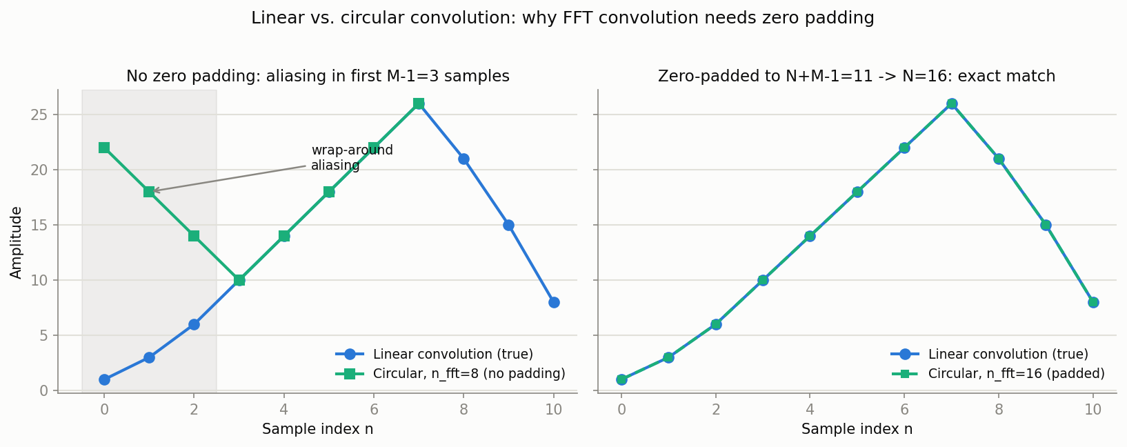
linear conv        : [ 1.  3.  6. 10. 14. 18. 22. 26. 21. 15.  8.]
circular (n_fft=8) : [22. 18. 14. 10. 14. 18. 22. 26.]
circular (n_fft=16): [ 1.  3.  6. 10. 14. 18. 22. 26. 21. 15.  8.]
max diff, no padding: 21.0
max diff, padded    : 1.7763568394002505e-15

Without zero padding (n_fft=8), the last three samples of the linear convolution (indices 8, 9, 10, with values 21, 15, 8) wrap around and add into the first three samples (indices 0, 1, 2) — e.g., 22 = 1 + 21, 18 = 3 + 15, 14 = 6 + 8 — with a maximum error as large as 21.0. Once zero-padded to satisfy \(N_{\text{fft}}=16 \ge L=11\) , the circular convolution matches the linear convolution to floating-point precision (\(\sim 10^{-15}\) ). This is shown below.

Correlation and the Matched Filter: A Numerical Experiment

We confirm the conclusion of equation \((6)\) — that the optimal filter for detecting a known waveform of unknown arrival time is correlation with the template — by detecting a pulse buried in noise.

import numpy as np
from scipy.signal import correlate

np.random.seed(7)
N = 2000
pulse = np.exp(-0.5 * (np.arange(-15, 16) / 4.0)**2)  # Gaussian pulse, length 31
true_delay = 823

signal = 0.6 * np.random.randn(N)
signal[true_delay:true_delay + len(pulse)] += pulse

# Matched filter = correlation with the known template
mf_output = correlate(signal, pulse, mode='same')
raw_argmax = np.argmax(mf_output)

print('true pulse center index :', true_delay + len(pulse)//2)
print('matched filter argmax   :', raw_argmax)
print('SNR before (peak/std)   :', pulse.max() / signal.std())
print('SNR after MF (peak/std) :', mf_output.max() / mf_output.std())

true pulse center index : 838
matched filter argmax   : 839
SNR before (peak/std)   : 1.675499480245094
SNR after MF (peak/std) : 4.836095661428964

The matched filter output peaks at index 839, off by only one sample from the true pulse center (index 838). Moreover, the raw SNR (peak amplitude over the standard deviation of the whole signal) is about 1.68, while the SNR after matched filtering rises to about 4.84 — roughly a 2.9x improvement. This is exactly the Cauchy–Schwarz equality condition (\(h[n] \propto s[K-1-n]\) ) from equation \((6)\) realized as this correlation operation.

Benchmarking Direct vs. FFT-Based Convolution

We measure the empirical crossover point between the direct method’s \(O(NM)\) and the FFT method’s \(O((N+M)\log(N+M))\) , sweeping the signal length.

import numpy as np
import time
from scipy.signal import fftconvolve

np.random.seed(42)
Ns = [8, 16, 32, 64, 128, 256, 512, 1024, 2048, 4096, 8192, 16384, 32768, 65536]

for N in Ns:
    x = np.random.randn(N)
    h = np.random.randn(N)  # square case, N=M
    reps = max(1, int(2000 / N))

    t0 = time.perf_counter()
    for _ in range(reps):
        y_direct = np.convolve(x, h, mode='full')
    t_direct = (time.perf_counter() - t0) / reps

    t0 = time.perf_counter()
    for _ in range(reps):
        y_fft = fftconvolve(x, h, mode='full')
    t_fft = (time.perf_counter() - t0) / reps

    print(f'{N:6d} | direct {t_direct*1e3:9.4f} ms | fft {t_fft*1e3:8.4f} ms | speedup {t_direct/t_fft:6.2f}x')

Measured results (NumPy 2.4 / SciPy 1.18):

     N=M | direct [ms] |  fft [ms] | speedup
       8 |      0.0010 |    0.0357 |   0.03x
      16 |      0.0011 |    0.0270 |   0.04x
      32 |      0.0014 |    0.0266 |   0.05x
      64 |      0.0022 |    0.0282 |   0.08x
     128 |      0.0045 |    0.0292 |   0.15x
     256 |      0.0128 |    0.0335 |   0.38x
     512 |      0.0422 |    0.1506 |   0.28x
    1024 |      0.1620 |    0.0808 |   2.00x
    2048 |      0.6563 |    0.1754 |   3.74x
    4096 |      2.6386 |    0.1340 |  19.70x
    8192 |     10.7775 |    0.3876 |  27.80x
   16384 |     50.5015 |    0.7445 |  67.84x
   32768 |    207.4742 |    1.5122 | 137.20x
   65536 |    852.2690 |    2.8904 | 294.86x

For \(N=M \le 512\) , the direct method is faster (the FFT’s fixed overhead dominates), but a crossover occurs around \(N=M=1024\) , after which the FFT method rapidly pulls ahead. At \(N=M=65536\) , we measure roughly a 295x speedup, matching the \(O(NM)\) vs. \(O(N\log N)\) theory. Since this crossover also depends on the kernel length \(M\) for practical FIR filtering (\(M \ll N\) ), SciPy provides scipy.signal.choose_conv_method, which automatically picks the faster method based on signal length, kernel length, and data type.

Overlap-Add and Overlap-Save

FFT convolution is fast, but when a signal is extremely long — streaming data, or data too large to fit in memory — computing a single giant FFT of length \(N_{\text{fft}} \approx N\) is inefficient or infeasible. Instead, we split the long signal into blocks, convolve each block with the short kernel \(h\) (length \(M\) ) via FFT, and stitch the results back together correctly.

• Overlap-Add (OLA): split the input into non-overlapping blocks of length \(L\) , and compute the length-\((L+M-1)\) FFT convolution of each block with \(h\) . Adjacent blocks’ outputs overlap by \(M-1\) samples; these overlapping tails are added together when concatenating.
• Overlap-Save (OLS): prepend the last \(M-1\) samples of the previous block to each block, compute a length-\(L\) circular convolution, and discard the first \(M-1\) samples (which are corrupted by aliasing), keeping only the valid remainder. No addition step is needed, but part of each block’s output is thrown away instead.

Both keep each individual FFT’s length around \(M\) , yet reproduce exactly the result of a single giant FFT overall. SciPy implements OLA as scipy.signal.oaconvolve.

import numpy as np
import time
from scipy.signal import fftconvolve, oaconvolve

np.random.seed(3)
N = 2_000_000   # long signal (e.g., streaming data)
M = 65          # short FIR kernel
x = np.random.randn(N)
h = np.random.randn(M)

t0 = time.perf_counter()
y_full_fft = fftconvolve(x, h, mode='full')
t_full = time.perf_counter() - t0

t0 = time.perf_counter()
y_oa = oaconvolve(x, h, mode='full')
t_oa = time.perf_counter() - t0

print('max abs diff:', np.max(np.abs(y_full_fft - y_oa)))
print(f'single-shot fftconvolve: {t_full*1e3:.1f} ms')
print(f'oaconvolve (block OLA) : {t_oa*1e3:.1f} ms')

max abs diff: 3.019806626980426e-14
single-shot fftconvolve: 66.5 ms
oaconvolve (block OLA) : 16.7 ms

The two outputs agree to floating-point precision (\(3.0 \times 10^{-14}\) ), confirming that block processing correctly reproduces linear convolution. Moreover, for this case where the kernel is extremely short relative to the signal (\(N=2{,}000{,}000\) , \(M=65\) ), the block-based OLA (16.7 ms) is roughly 4x faster than the single giant FFT (66.5 ms). A single FFT of length \(N_{\text{fft}} \approx N\) is memory-bandwidth bound, whereas OLA with a well-chosen block size repeats many small, cache-resident FFTs, raising effective throughput.

Connection to the Moving Average

A simple moving average (SMA) of length \(L\) is a convolution with the box window \(h_{\text{box}}[n]\) whose coefficients are all \(1/L\) :

import numpy as np
import matplotlib.pyplot as plt

np.random.seed(1)
fs = 1000
t = np.arange(0, 1, 1/fs)
signal = np.sin(2*np.pi*5*t) + 0.4*np.random.randn(len(t))

L = 21
h_box = np.ones(L) / L

# Moving average = convolution with the box window
sma = np.convolve(signal, h_box, mode='same')

# Cross-check with scipy.ndimage.uniform_filter1d
from scipy.ndimage import uniform_filter1d
sma_ref = uniform_filter1d(signal, size=L, mode='nearest')

plt.figure(figsize=(10, 4))
plt.plot(t, signal, alpha=0.4, label='Noisy signal')
plt.plot(t, sma, label=f'Convolution with box (L={L})')
plt.plot(t, sma_ref, '--', label='uniform_filter1d (reference)')
plt.xlabel('Time [s]')
plt.ylabel('Amplitude')
plt.legend()
plt.grid(True, alpha=0.3)
plt.tight_layout()
plt.show()

Up to boundary handling, both outputs coincide, confirming that the moving average is a special case of convolution. Replacing the kernel by a triangular or Hann window naturally extends the idea to more general FIR filters.

Beyond the Basics: The Convolution Theorem’s Resurgence in Deep Learning (2023 Onward)

The convolution theorem is nearly a century old, but since 2023 it has been re-examined by deep learning researchers as a way to sidestep the \(O(L^2)\) cost (quadratic in sequence length \(L\) ) of Transformer self-attention.

Gu et al.’s S4 (Structured State Space Sequence model) (2022, ICLR) applies a global convolution kernel derived from a state-space model via the FFT, capturing dependencies across an entire sequence in \(O(L \log L)\) . Building on this, Hyena Hierarchy (Poli et al., ICML 2023) replaces self-attention entirely with a combination of implicitly parameterized long convolutions and multiplicative gating. It reports matching a highly optimized attention implementation at sequence length 8,192 and running roughly 100x faster at sequence length 65,536. On reasoning tasks over tens of thousands to hundreds of thousands of tokens, it improves accuracy by more than 50 points over prior subquadratic approaches (state-space models and others), and it sets a new state of the art among dense-attention-free architectures on standard language modeling benchmarks (WikiText103, The Pile).

However, the FFT convolution of equation \((10)\) requires three FFTs (two forward, one inverse) plus an elementwise product — several memory-bound kernel launches — so on GPUs its theoretical complexity advantage historically failed to translate directly into wall-clock speedups. FlashFFTConv (Fu et al., 2023) addresses this by rewriting the FFT as a sequence of matrix multiplications via a Monarch decomposition and fusing the kernels so they run on GPU tensor cores, reporting up to a 7.93x speedup over PyTorch’s native FFT convolution and up to 4.4x end-to-end. This translated into a 2.3-point perplexity improvement for Hyena-GPT-s, a 3.3-point GLUE score improvement for M2-BERT-base, and 96.1% accuracy on the high-resolution vision task Path-512, where no prior model had exceeded 50%.

The classical facts derived in this article — that the convolution theorem lets us accelerate convolution via the FFT, and that zero padding is required to correctly compute linear (rather than circular) convolution — appear in essentially the same form inside the implementations of these state-of-the-art sequence models.

Summary

• Convolution flips one signal, slides it, and accumulates the elementwise product; it fully describes any LTI system response.
• The convolution theorem \(\mathcal{F}\{x \circledast h\} = X \cdot H\) (equation \((8)\) ) can be proven directly from the definitions via a change of variables — a translation \(u=t-\tau\) in continuous time, a circular shift mod \(N\) for the discrete DFT.
• The DFT convolution theorem holds for circular convolution; matching it to linear convolution requires zero-padding to \(N_{\text{fft}} \ge N+M-1\) . Insufficient padding causes aliasing in the early samples (our experiment showed a maximum error of 21.0, dropping to \(\sim 10^{-15}\) once properly padded).
• Correlation is similar but without the time reversal: cross-correlation \(R_{xy}\) enables template matching, while auto-correlation \(R_{xx}\) uncovers periodic structure. The Cauchy–Schwarz inequality rigorously shows that the optimal filter for detecting a known waveform at maximum SNR — the matched filter — is exactly the correlation operation.
• The empirical crossover between direct convolution (\(O(NM)\) ) and FFT convolution (\(O((N+M)\log(N+M))\) ) occurs around \(N=M\approx 1024\) ; at \(N=M=65536\) the FFT method is about 295x faster.
• For extremely long signals, overlap-add / overlap-save split FFT convolution into blocks; in our experiment this was about 4x faster than a single giant FFT.
• Moving average filters are convolutions with a box window — the simplest FIR filter.
• Wiener–Khinchin shows that auto-correlation and PSD are two views of the same quantity.
• Since 2023, the convolution theorem and the FFT have been re-evaluated as core technology behind subquadratic-time sequence modeling approaches — such as Hyena Hierarchy and FlashFFTConv — that aim to replace Transformer self-attention.

Mastering these primitives makes filter design, spectral analysis, and time-frequency analysis feel like one coherent mathematical framework.

Related Posts

• Fast Fourier Transform (FFT): Theory and Python Implementation — The DFT/FFT foundation underlying the convolution theorem.
• Window Functions and Power Spectral Density (PSD): Theory and Python Implementation — PSD estimation built on the auto-correlation / Wiener–Khinchin perspective.
• Wavelet Transform: Theory and Python Implementation — A convolution-based time-frequency extension of FFT.
• Comparison of Moving Average Filters — Frames SMA/WMA/EMA through the convolution-with-a-window lens.
• Autocorrelation and Cross-Correlation: Theory and Python Implementation — Builds on the correlation definitions here for ACF/PACF time-series analysis and delay estimation (GCC-PHAT).
• Cepstrum Analysis: Theory and Python Implementation — A canonical application that factors convolution through the log spectrum, enabling F0 estimation and spectral envelope analysis.
• FIR and IIR Filter Comparison — Contrasts FIR filters that implement convolution directly with the recursive structure of IIR filters.
• Understanding DTFT, DFT, and FFT — Organizes the hierarchy of frequency transforms (DTFT, DFT) in which the convolution theorem holds, complementing the theory behind FFT-based convolution.

References

• Oppenheim, A. V., & Schafer, R. W. (2009). Discrete-Time Signal Processing (3rd ed.). Prentice Hall.
• Smith, S. W. (1997). The Scientist and Engineer’s Guide to Digital Signal Processing. California Technical Publishing.
• Gu, A., Goel, K., & Ré, C. (2022). Efficiently Modeling Long Sequences with Structured State Spaces. ICLR 2022.
• Poli, M., Massaroli, S., Nguyen, E., et al. (2023). Hyena Hierarchy: Towards Larger Convolutional Language Models. ICML 2023. arXiv:2302.10866
• Fu, D. Y., Kumbong, H., Nguyen, E., & Ré, C. (2023). FlashFFTConv: Efficient Convolutions for Long Sequences with Tensor Cores. arXiv:2311.05908
• NumPy convolve documentation
• SciPy signal documentation