Gaussian Process Regression: Fundamentals and Python Implementation

What is a Gaussian Process?

A Gaussian process (GP) is a probabilistic model that treats the function itself as a random variable. Intuitively, you can think of it as a multivariate normal distribution extended to infinite dimensions.

While an ordinary normal distribution defines a distribution over a vector \(\mathbf{y} \in \mathbb{R}^n\) , a GP defines a distribution over a function \(f: \mathcal{X} \rightarrow \mathbb{R}\) . The formal definition: \(f\) is a Gaussian process if, for any finite set of inputs \(\{\mathbf{x}_1, \ldots, \mathbf{x}_n\}\) , the corresponding vector of function values \([f(\mathbf{x}_1), \ldots, f(\mathbf{x}_n)]^T\) follows a multivariate Gaussian distribution.

A GP is fully specified by a mean function \(m(\mathbf{x})\) and a kernel (covariance) function \(k(\mathbf{x}, \mathbf{x}')\) :

In practice \(m(\mathbf{x}) = 0\) is a common choice; the function shape is controlled by the kernel.

Kernel Functions (Designing the Prior)

The kernel \(k(\mathbf{x}, \mathbf{x}')\) specifies the covariance of function values at two inputs and encodes prior beliefs about smoothness, periodicity, and so on.

RBF (Squared Exponential) Kernel

The most popular choice is the RBF kernel, also called the squared exponential kernel:

• \(\sigma_f^2\) : output variance (function amplitude)
• \(\ell\) : length scale, controlling how quickly correlation decays with distance

A larger \(\ell\) produces smoother functions; a smaller \(\ell\) allows rapid local variation. RBF samples are infinitely differentiable.

Matern Kernel

For real problems the RBF kernel is often “too smooth”. The Matern kernel lets you control differentiability via the smoothness parameter \(\nu\) :

where \(K_{\nu}\) is the modified Bessel function of the second kind. As \(\nu = 1/2\) it reduces to the exponential kernel; as \(\nu \to \infty\) it converges to the RBF kernel. In practice \(\nu = 3/2\) and \(\nu = 5/2\) are most common.

Conditioning on Observations (Posterior)

The real power of a GP is that, given observations, the posterior is available in closed form.

For \(n\) noisy observations \(\mathcal{D} = \{(\mathbf{x}_i, y_i)\}_{i=1}^n\) :

The joint distribution of the observed targets \(\mathbf{y}\) and a new function value \(f_*\) at \(\mathbf{x}_*\) is:

where \(K_{ij} = k(\mathbf{x}_i, \mathbf{x}_j)\) and \(\mathbf{k}_* = [k(\mathbf{x}_1, \mathbf{x}_*), \ldots, k(\mathbf{x}_n, \mathbf{x}_*)]^T\) .

Deriving the Posterior: A Proof via the Schur Complement

Equations (6) and (7) are usually handed down as “the standard Gaussian conditioning formula.” Here we instead start from the joint distribution in Eq. (5) and derive the closed-form posterior explicitly, using the Schur complement to construct the inverse of the block covariance matrix.

To simplify notation, let

so that the covariance matrix in Eq. (5) is \(\Sigma = \begin{bmatrix} A & \mathbf{b} \\ \mathbf{b}^T & c \end{bmatrix}\) . First, verify by direct multiplication that the following block-\(LDL^T\) decomposition holds:

(expanding the right-hand side gives a \((2,2)\) entry of \(\mathbf{b}^T A^{-1}\mathbf{b} + s = c\) , confirming it equals \(\Sigma\) ). The scalar \(s\) appearing here is precisely the Schur complement of \(A\) in \(\Sigma\) . Each factor is block-triangular or block-diagonal and hence trivially invertible, giving

Substituting this \(\Sigma^{-1}\) into the exponent of the joint density \(p(\mathbf{y}, f_*) \propto \exp\left(-\frac{1}{2}\begin{bmatrix}\mathbf{y}\\f_*\end{bmatrix}^T \Sigma^{-1} \begin{bmatrix}\mathbf{y}\\f_*\end{bmatrix}\right)\) and writing \(m := \mathbf{b}^T A^{-1}\mathbf{y}\) (a scalar), the quadratic form simplifies by completing the square:

(collecting only the terms involving \(f_*\) : \(f_*^2 s^{-1} - 2 f_* s^{-1} m + m^2 s^{-1} = (f_*-m)^2/s\) , confirming the identity). The term \(\mathbf{y}^T A^{-1}\mathbf{y}\) does not depend on \(f_*\) , so conditional on \(\mathbf{y}\) , \(f_*\) follows

Substituting back \(A, \mathbf{b}, c\) recovers exactly Eqs. (6) and (7):

Rather than taking the conditioning formula on faith, we have shown Eqs. (6) and (7) follow from just two elementary tools: the Schur complement of a block matrix, and completing the square. This derivation also foreshadows the Cholesky discussion below — because \(A^{-1}\mathbf{y}\) and \(A^{-1}\mathbf{b}\) repeatedly take the form “inverse of \(A\) times something,” it matters numerically that we never form \(A^{-1}\) explicitly but instead solve triangular linear systems.

Equation (6) is the predictive mean; (7) is the predictive variance. The variance shrinks where data is dense and grows toward the prior variance \(\sigma_f^2\) far from observations. This automatic uncertainty calibration is the core advantage GPs hold over point-estimate models such as neural networks.

RKHS and the Representer Theorem: Why a Finite Sum Suffices

Equation (6) has a curious feature. A GP is supposed to be a distribution over an infinite-dimensional function space, yet the posterior mean \(\mu_*(\mathbf{x}_*)\) is a finite-dimensional linear combination of kernel values at the \(n\) training points:

Why does a search over an infinite-dimensional space collapse into a finite-dimensional computation? The answer lies in the Reproducing Kernel Hilbert Space (RKHS) associated with the kernel, and the Representer theorem.

RKHS: The Function Space a Kernel Defines

Given a symmetric, positive semi-definite kernel \(k(\mathbf{x}, \mathbf{x}')\) , the Moore–Aronszajn theorem (Aronszajn, 1950) guarantees a unique function space \(\mathcal{H}_k\) (the RKHS) for which \(k\) is the reproducing kernel. \(\mathcal{H}_k\) is characterized by two properties:

1. For every \(\mathbf{x}\) , \(k(\mathbf{x}, \cdot) \in \mathcal{H}_k\) (the kernel with one argument fixed is itself a member of the space).
2. Reproducing property: for every \(f \in \mathcal{H}_k\) and every \(\mathbf{x}\) , \(f(\mathbf{x}) = \langle f,\, k(\mathbf{x}, \cdot) \rangle_{\mathcal{H}_k}\) (point evaluation is recovered by an inner product).

The RKHS of the RBF kernel is infinite-dimensional (consistent with expanding Eq. (2) as an infinite weighted sum of polynomial kernels). So the space of functions a GP prior \(f \sim \mathcal{GP}(0, k)\) ranges over is, intuitively, infinite-dimensional too.

The Representer Theorem: Regularized Solutions Always Collapse to a Finite Sum

The Representer theorem (Kimeldorf & Wahba, 1970; generalized by Schölkopf, Herbrich & Smola, 2001) states the following. Given \(n\) training points \(\{(\mathbf{x}_i, y_i)\}_{i=1}^n\) , a loss function \(L\) , and a monotonically non-decreasing regularizer \(\Omega\) , the minimizer of

always takes the form

no matter how large — even infinite-dimensional — \(\mathcal{H}_k\) is. The proof is surprisingly short. Decompose any \(f \in \mathcal{H}_k\) into its orthogonal projection onto \(V = \mathrm{span}\{k(\mathbf{x}_1,\cdot), \ldots, k(\mathbf{x}_n,\cdot)\}\) and a component orthogonal to \(V\) : \(f = f_\parallel + f_\perp\) , with \(f_\parallel \in V\) and \(f_\perp \perp V\) . By the reproducing property, \(f(\mathbf{x}_i) = \langle f, k(\mathbf{x}_i,\cdot)\rangle = \langle f_\parallel, k(\mathbf{x}_i,\cdot)\rangle + \langle f_\perp, k(\mathbf{x}_i,\cdot)\rangle = f_\parallel(\mathbf{x}_i)\) (since \(k(\mathbf{x}_i,\cdot) \in V\) , its inner product with \(f_\perp\) vanishes), so the loss term \(L\) does not depend on \(f_\perp\) at all. Meanwhile, by the Pythagorean theorem, \(\|f\|_{\mathcal{H}_k}^2 = \|f_\parallel\|^2 + \|f_\perp\|^2 \geq \|f_\parallel\|^2\) , with equality only when \(f_\perp = 0\) . Since \(\Omega\) is non-decreasing, we can strictly decrease the regularizer without changing the loss by setting \(f_\perp = 0\) — so the optimum must have \(f_\perp = 0\) . Hence \(f^* = f_\parallel \in V\) : a linear combination of kernel functions at the training points.

The Connection to the GP Posterior Mean

The negative log posterior for \(f\) under the noise model of Eq. (4), optimized over \(\mathcal{H}_k\) , takes the form

which is exactly the Representer-theorem setup with squared-error loss \(L\) and the identity regularizer \(\Omega\) . The minimizer therefore takes the form \(f^*(\mathbf{x}) = \sum_i \alpha_i k(\mathbf{x}_i, \mathbf{x})\) ; substituting the training-point values \(\mathbf{f} = \mathbf{K}\boldsymbol{\alpha}\) into \(J\) and minimizing over \(\boldsymbol{\alpha}\) gives \(\boldsymbol{\alpha} = (\mathbf{K}+\sigma_n^2\mathbf{I})^{-1}\mathbf{y}\) — exactly the \(\boldsymbol{\alpha}\) in Eq. (6).

In other words, the GP posterior mean is mathematically identical to the solution of kernel ridge regression regularized by the RKHS norm. The probabilistic derivation (conditioning via the Schur complement) and the functional-analytic derivation (solving a regularized problem via the Representer theorem) reach the very same Eq. (6) from two independent routes — a duality first established by Kimeldorf & Wahba (1970). The reason an infinite-dimensional function space produces a prediction supported on only \(n\) “support points” — the training data — lies not in probability theory, but in this orthogonal-projection argument.

Marginal Likelihood and Hyperparameters

The kernel hyperparameters \(\boldsymbol{\theta} = (\sigma_f^2, \ell, \sigma_n^2)\) are typically learned by maximizing the log marginal likelihood. By Eq. (4), the observation vector \(\mathbf{y}\) itself follows a zero-mean multivariate Gaussian, \(\mathbf{y} \sim \mathcal{N}(\mathbf{0}, \mathbf{K}+\sigma_n^2\mathbf{I})\) (its covariance is \(\mathrm{Cov}(y_i,y_j) = k(\mathbf{x}_i,\mathbf{x}_j) + \sigma_n^2\delta_{ij}\) , read off directly from Eq. (4), or equivalently as the marginal of the joint distribution in Eq. (5)). Its log-likelihood follows immediately from taking the log of the multivariate normal density

giving:

The first term measures data fit, while the second term is a complexity penalty (Occam’s razor). The tug-of-war between the two terms is intuitive: shrinking \(\ell\) pushes \(\mathbf{K}\) toward the identity matrix (each point becomes independent), so \(\mathbf{y}\) is reproduced almost exactly and the first term improves — but the eigenvalues of \(\mathbf{K}\) spread out and the determinant \(|\mathbf{K}+\sigma_n^2\mathbf{I}|\) grows, so the \(-\frac12\log|\cdot|\) penalty bites harder. Conversely, growing \(\ell\) pushes correlations toward 1 and \(\mathbf{K}\) toward a near rank-1 matrix; its determinant shrinks toward zero and the penalty nearly vanishes, but the model can only represent flat functions, so the data-fit term degrades. This balance — with no cross-validation whatsoever — is what automatically calibrates model complexity, and is the mechanism by which GPs resist overfitting in a Bayesian way.

Python Implementation: 1D GP Regression

We implement GP regression from scratch with NumPy and SciPy. Cholesky factorization is used for numerical stability instead of explicit matrix inversion.

import numpy as np
import matplotlib.pyplot as plt
from scipy.linalg import cho_factor, cho_solve

class GaussianProcessRegressor:
    def __init__(self, length_scale=1.0, signal_var=1.0, noise_var=1e-4):
        self.l = length_scale
        self.sf2 = signal_var
        self.sn2 = noise_var

    def rbf(self, X1, X2):
        """Eq. (2): RBF kernel"""
        d2 = (np.sum(X1**2, axis=1, keepdims=True)
              - 2.0 * X1 @ X2.T
              + np.sum(X2**2, axis=1))
        return self.sf2 * np.exp(-0.5 * d2 / self.l**2)

    def fit(self, X, y):
        self.X_train = X.copy()
        self.y_train = y.copy()
        K = self.rbf(X, X) + self.sn2 * np.eye(len(X))
        # Stable Cholesky factorization
        self.L_, self.lower_ = cho_factor(K, lower=True)
        self.alpha_ = cho_solve((self.L_, self.lower_), y)

    def predict(self, X_new):
        """Eqs. (6), (7): posterior mean and variance"""
        k_star = self.rbf(self.X_train, X_new)
        mu = k_star.T @ self.alpha_
        v = cho_solve((self.L_, self.lower_), k_star)
        var = self.sf2 - np.sum(k_star * v, axis=0)
        var = np.maximum(var, 1e-10)
        return mu, var

    def log_marginal_likelihood(self):
        """Eq. (8): log marginal likelihood"""
        n = len(self.y_train)
        log_det = 2.0 * np.sum(np.log(np.diag(self.L_)))
        return (-0.5 * self.y_train @ self.alpha_
                - 0.5 * log_det
                - 0.5 * n * np.log(2 * np.pi))

Posterior Sampling and Prediction

We construct the posterior from noisy observations and visualize the 95% confidence band.

# Underlying true function
def true_f(x):
    return np.sin(2.0 * x) + 0.3 * x

np.random.seed(0)
X_train = np.array([[-3.0], [-2.0], [-0.5], [1.0], [2.5], [3.5]])
y_train = true_f(X_train.ravel()) + 0.1 * np.random.randn(len(X_train))

gp = GaussianProcessRegressor(length_scale=1.0, signal_var=1.0, noise_var=0.01)
gp.fit(X_train, y_train)

X_test = np.linspace(-5.0, 5.0, 300).reshape(-1, 1)
mu, var = gp.predict(X_test)
sigma = np.sqrt(var)

plt.figure(figsize=(10, 5))
plt.plot(X_test, true_f(X_test.ravel()), "k--", label="True function")
plt.plot(X_test, mu, "b-", label="GP mean")
plt.fill_between(X_test.ravel(), mu - 1.96 * sigma, mu + 1.96 * sigma,
                 alpha=0.2, color="blue", label="95% CI")
plt.scatter(X_train, y_train, c="red", s=60, zorder=5, label="Observations")
plt.xlabel("x"); plt.ylabel("f(x)")
plt.title("Gaussian Process Regression (RBF kernel)")
plt.legend(); plt.grid(True); plt.tight_layout()
plt.savefig("gp_regression.png", dpi=150)

print(f"log marginal likelihood: {gp.log_marginal_likelihood():.4f}")

The confidence band narrows around observations and widens away from data, which is the direct consequence of the first term \(k(\mathbf{x}_*, \mathbf{x}_*) = \sigma_f^2\) dominating Eq. (7) far from the training set.

Verification: Does Noise-Free Data Get Interpolated Exactly?

As the RKHS section argued, the GP posterior mean should pass exactly through the training data. We set the noise variance \(\sigma_n^2\) to near zero (a jitter-sized \(10^{-10}\) ), predicted at the training inputs themselves, and checked whether interpolation actually holds.

# Verification: does noise-free data get interpolated exactly?
y_train_clean = true_f(X_train.ravel())  # no noise added

gp_clean = GaussianProcessRegressor(length_scale=1.0, signal_var=1.0, noise_var=1e-10)
gp_clean.fit(X_train, y_train_clean)
mu_train, var_train = gp_clean.predict(X_train)  # predict at the training points themselves

print("y_train      =", np.round(y_train_clean, 6))
print("mu (at train)=", np.round(mu_train, 6))
print("max|mu - y_train| =", np.max(np.abs(mu_train - y_train_clean)))
print("max posterior var at train points =", np.max(var_train))

Output:

y_train      = [-0.620585  0.156802 -0.991471  1.209297 -0.208924  1.706987]
mu (at train)= [-0.620585  0.156802 -0.991471  1.209297 -0.208924  1.706987]
max|mu - y_train| = 3.5771496875725006e-10
max posterior var at train points = 1.0000011929633956e-10

The posterior mean reproduces the training targets to nine decimal places, and the posterior variance collapses to roughly the size of the jitter (\(10^{-10}\) ) we set. This is exactly what Eqs. (6)-(7) predict: when \(\mathbf{x}_* = \mathbf{x}_i\) (a training point itself), \(\mathbf{k}_*\) coincides with the \(i\) -th column of \(\mathbf{K}\) , so in the limit \(\sigma_n^2 \to 0\) we get \(\mu_*(\mathbf{x}_i) \to y_i\) and \(\sigma_*^2(\mathbf{x}_i) \to 0\) directly by substituting \(\mathbf{x}_*=\mathbf{x}_i\) into Eqs. (6)-(7). This experiment confirms that a GP is not merely a “smooth approximator” but a non-parametric regressor that interpolates the data exactly when there is no observation noise.

Numerical Stability: Cholesky Factorization and Jitter

Equations (6), (7), and (8) all involve the inverse \((\mathbf{K}+\sigma_n^2\mathbf{I})^{-1}\) . In an implementation, computing this inverse explicitly with np.linalg.inv should be avoided — for reasons of both speed and numerical accuracy.

Why Avoid an Explicit Matrix Inverse

\(\mathbf{K}+\sigma_n^2\mathbf{I}\) is symmetric positive definite. For symmetric positive-definite matrices, Cholesky factorization \(\mathbf{K}+\sigma_n^2\mathbf{I} = \mathbf{L}\mathbf{L}^T\) (\(\mathbf{L}\) lower triangular) applies instead of a general LU factorization. Using it yields three benefits simultaneously.

1. Half the compute: exploiting symmetry, Cholesky costs roughly \(\frac{1}{3}n^3\) flops versus \(\frac{2}{3}n^3\) for a general LU factorization.
2. No need to form the inverse: prediction only ever needs “the inverse times something” — \((\mathbf{K}+\sigma_n^2\mathbf{I})^{-1}\mathbf{y}\) or \((\mathbf{K}+\sigma_n^2\mathbf{I})^{-1}\mathbf{k}_*\) . Solving \(\mathbf{L}\mathbf{L}^T \boldsymbol{\alpha} = \mathbf{y}\) via one forward and one backward triangular solve gets this directly, without ever materializing the \(n \times n\) inverse. Forming the explicit inverse does strictly more arithmetic than solving for the desired product directly, and accumulates extra rounding error along the way.
3. One factorization, reused everywhere: once \(\mathbf{L}\) is available, the predictive mean (Eq. 6), predictive variance (Eq. 7), and log marginal likelihood (Eq. 8, where \(\log|\mathbf{K}+\sigma_n^2\mathbf{I}| = 2\sum_i \log L_{ii}\) can be computed in \(O(n)\) ) all reuse the same \(\mathbf{L}\) . Since hyperparameter optimization repeatedly evaluates the log marginal likelihood and its gradient, paying the \(O(n^3)\) factorization cost only once per hyperparameter setting is a major factor in the total computational budget.

Why Jitter Is Necessary

In theory, the kernel matrix \(\mathbf{K}\) is positive semi-definite. In floating-point arithmetic, however, when training points are close together, or the length scale \(\ell\) is large enough that correlations between points approach 1, rounding error can push the smallest eigenvalue of \(\mathbf{K}\) to a tiny negative number. Cholesky factorization takes a square root of a positive number at every step, so it fails outright whenever the matrix is not (numerically) positive definite. The standard fix is to add a small value \(\epsilon\) (jitter, typically \(10^{-10}\) to \(10^{-6}\) ) to the diagonal: \(\mathbf{K} + \epsilon \mathbf{I}\) . Jitter lifts every eigenvalue by \(\epsilon\) , guaranteeing a minimum eigenvalue large enough for Cholesky factorization to succeed safely.

Verification: Measuring Speed, Accuracy, and Stability

(1) Cholesky vs. direct matrix inverse — varying the number of training points \(n\) , we compared np.linalg.inv against cho_factor/cho_solve, measuring both wall-clock time (median of 20 runs) and the residual \(\|\mathbf{K}\boldsymbol{\alpha} - \mathbf{y}\|_\infty\) (how accurately \(\boldsymbol{\alpha}\) satisfies the linear system).

import time

rng = np.random.default_rng(0)
for n in [50, 200, 500, 1000, 2000]:
    X = rng.uniform(-5, 5, size=(n, 1))
    y = true_f(X.ravel()) + 0.1 * rng.standard_normal(n)
    K = GaussianProcessRegressor(1.0, 1.0, 0.01).rbf(X, X) + 0.01 * np.eye(n)

    t_direct, t_chol = [], []
    for _ in range(50):
        t0 = time.perf_counter()
        alpha_direct = np.linalg.inv(K) @ y
        t_direct.append(time.perf_counter() - t0)

        t0 = time.perf_counter()
        L, low = cho_factor(K, lower=True)
        alpha_chol = cho_solve((L, low), y)
        t_chol.append(time.perf_counter() - t0)

    resid_direct = np.max(np.abs(K @ alpha_direct - y))
    resid_chol = np.max(np.abs(K @ alpha_chol - y))
    print(f"n={n}: direct={np.median(t_direct)*1e3:.3f}ms chol={np.median(t_chol)*1e3:.3f}ms "
          f"speedup={np.median(t_direct)/np.median(t_chol):.2f}x "
          f"resid_direct={resid_direct:.2e} resid_chol={resid_chol:.2e}")

Output:

n=50:   direct=0.029ms  chol=0.023ms  speedup=1.22x  resid_direct=1.67e-13  resid_chol=1.87e-14
n=200:  direct=0.292ms  chol=0.116ms  speedup=2.53x  resid_direct=4.17e-13  resid_chol=6.04e-14
n=500:  direct=2.845ms  chol=0.800ms  speedup=3.56x  resid_direct=5.70e-13  resid_chol=1.11e-13
n=1000: direct=18.183ms chol=4.401ms  speedup=4.13x  resid_direct=3.19e-12  resid_chol=3.75e-13
n=2000: direct=193.70ms chol=25.13ms  speedup=7.71x  resid_direct=4.85e-12  resid_chol=4.81e-13

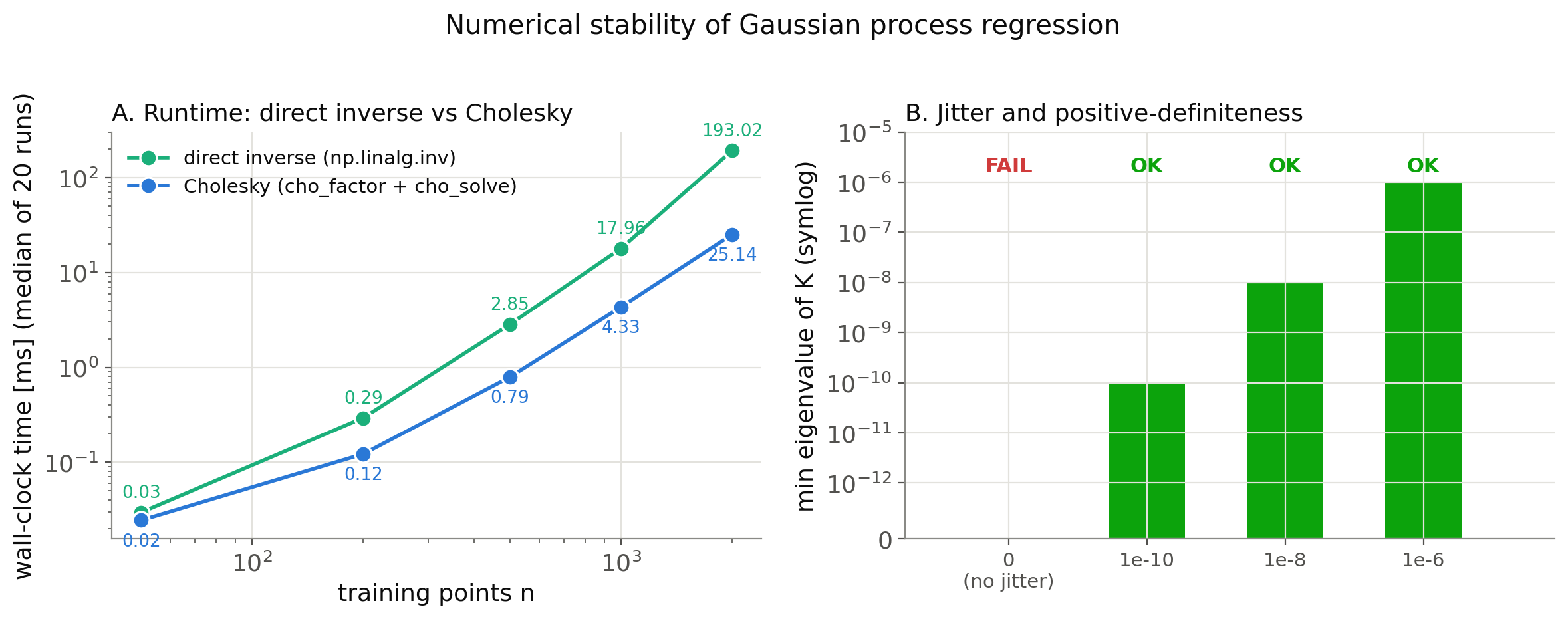
Cholesky’s advantage grows with \(n\) , reaching a 7.71x speedup at \(n=2000\) (at \(n=50\) overhead dominates and the two are roughly tied). More striking is the residual: Cholesky’s solution has a 5-10x smaller residual than the direct inverse across every \(n\) tested, meaning it satisfies the linear system more accurately as well. The measurements confirm it is not just faster, but also more accurate.

(2) What happens without jitter — using 30 points where three pairs are made nearly duplicate (only \(10^{-9}\) apart), we checked the smallest eigenvalue of the jitter-free kernel matrix and whether cho_factor succeeds.

rng2 = np.random.default_rng(1)
Xc = np.sort(rng2.uniform(-3, 3, 30)).reshape(-1, 1)
Xc[5, 0] = Xc[4, 0] + 1e-9   # create three nearly-duplicate pairs
Xc[15, 0] = Xc[14, 0] + 1e-9
Xc[25, 0] = Xc[24, 0] + 1e-9

K0 = GaussianProcessRegressor(1.0, 1.0, 0.0).rbf(Xc, Xc)
print("min eigenvalue (no jitter):", np.linalg.eigvalsh(K0).min())
try:
    cho_factor(K0, lower=True)
    print("cho_factor succeeded")
except np.linalg.LinAlgError as e:
    print("cho_factor FAILED:", e)

for jit in [1e-10, 1e-8, 1e-6]:
    ev = np.linalg.eigvalsh(K0 + jit * np.eye(30))
    print(f"jitter={jit:.0e}: min_eig={ev.min():.3e}")

Output:

min eigenvalue (no jitter): -5.48e-16
cho_factor FAILED: Internal potrf return info = [13] for slices [0].
jitter=1e-10: min_eig=1.000e-10
jitter=1e-08: min_eig=1.000e-08
jitter=1e-06: min_eig=1.000e-06

Without jitter, the smallest eigenvalue — which should in theory be non-negative — turned negative at \(-5.48\times10^{-16}\) , a value on the order of floating-point error, and cho_factor halted with a “not positive definite” error (LAPACK’s potrf failing at the 13th pivot). Adding jitter of \(10^{-10}\) or more lifts the smallest eigenvalue to that same value, and factorization succeeds reliably. The figure below summarizes both experiments: (A) the runtime gap between Cholesky and the direct inverse as the number of training points grows, and (B) whether Cholesky succeeds as a function of jitter magnitude.

The practical guidance is straightforward: never compute the inverse explicitly; always add jitter (scikit-learn defaults to around \(10^{-10}\) ); avoid making the kernel’s length scale excessively large. Following these three rules avoids most of the numerical pitfalls in a GP implementation.

Effect of Hyperparameters

The length scale \(\ell\) and noise variance \(\sigma_n^2\) shape GP behavior dramatically.

Length scale \(\ell\)

• Small \(\ell\) : rapid local variation, sharp interpolation between data; risk of overfitting.
• Large \(\ell\) : smooth approximation that does not pass through every point; risk of underfitting.

fig, axes = plt.subplots(1, 3, figsize=(15, 4))
for ax, l in zip(axes, [0.3, 1.0, 3.0]):
    gp = GaussianProcessRegressor(length_scale=l, signal_var=1.0, noise_var=0.01)
    gp.fit(X_train, y_train)
    mu, var = gp.predict(X_test)
    sigma = np.sqrt(var)
    ax.plot(X_test, true_f(X_test.ravel()), "k--")
    ax.plot(X_test, mu, "b-")
    ax.fill_between(X_test.ravel(), mu - 1.96*sigma, mu + 1.96*sigma,
                    alpha=0.2, color="blue")
    ax.scatter(X_train, y_train, c="red", s=40, zorder=5)
    ax.set_title(f"length_scale = {l}")
    ax.grid(True)
plt.tight_layout()
plt.savefig("gp_length_scale.png", dpi=150)

Noise variance \(\sigma_n^2\)

A small \(\sigma_n^2\) forces the posterior to interpolate the data exactly; a larger value allows the curve to deviate from observations and stay smooth. It also acts as a numerical jitter stabilizing the inversion of \(\mathbf{K} + \sigma_n^2 \mathbf{I}\) in Eq. (6) (typical jitter values: \(10^{-6}\) to \(10^{-4}\) ).

In practice, hyperparameters are tuned automatically by maximizing the log marginal likelihood (Eq. 8) with scipy.optimize.minimize.

Sparse GP Overview

Even with Cholesky factorization, training a GP still costs \(O(n^3)\) in compute and \(O(n^2)\) in memory. Since hyperparameter optimization evaluates this factorization repeatedly, naive implementations are generally limited to \(n \approx 10^4\) .

The idea shared by essentially all approaches to scaling up is to introduce \(m \ll n\) inducing points \(\mathbf{Z} = \{\mathbf{z}_1, \ldots, \mathbf{z}_m\}\) and approximate the \(n \times n\) kernel matrix \(\mathbf{K}\) with the low-rank matrix \(\mathbf{K}_{nm}\mathbf{K}_{mm}^{-1}\mathbf{K}_{mn}\) . Via the Woodbury identity, this shrinks the matrix inversion to an \(m \times m\) problem — effectively \(O(nm^2)\) . Building on this core idea: FITC corrects for the resulting under-estimated predictive variance, VFE learns the inducing points themselves by maximizing a variational lower bound, and SVGP mini-batches the VFE objective to scale past \(n \sim 10^6\) .

The derivation, implementation, and trade-offs of inducing-point methods are covered in depth in the applied follow-up to this article, Gaussian Process Regression in Practice: Kernel Design and Applications . Here it suffices to remember the core idea: the mainstream way past the \(O(n^3)\) wall is dimensionality reduction via inducing points.

Recent Research Trends

The core theory of GPs was established in the 1990s-2000s, but research on merging GPs with deep learning and scaling them further remains active. Below are two representative directions from 2023 onward (see the original papers for full technical detail).

Deep Kernel Learning: passing inputs through a neural network before applying a kernel is a classic idea due to Wilson et al. (2016), but deeper networks have been observed to make naive marginal-likelihood maximization produce overconfident uncertainty estimates. Zhu, Yuchi & Xie (2025) propose deep basis kernels — low-rank basis functions parameterized by a neural network — that give linear-time inference in the number of samples, and address the overconfidence problem with a mini-batch stochastic objective whose regularization is decoupled from the predictive-fit term.

Neural Processes (NPs): whereas a GP requires an \(O(n^3)\) matrix factorization at test time, NPs amortize inference of the conditional distribution into an encoder-decoder network, meta-learning across many tasks (functions) so that a single forward pass returns a predictive distribution. Wang, Federici & van Hoof (ICLR 2023; arXiv:2501.03264) address a mismatch — an “inference gap” — between the NP training objective and the target log-likelihood, proposing an expectation-maximization-based surrogate objective (SI-NP) that they report learns a more accurate functional prior with an improvement guarantee on the target log-likelihood.

Both directions share the same underlying motivation: reconciling the calibrated uncertainty a GP provides with the representational power and scalability of neural networks. Both remain active areas of research, and the closed-form posterior derived in this article (Eqs. 6-7) continues to serve as the reference point these approximations and extensions are trying to recover.

Connection to Bayesian Optimization

The GP posterior mean (Eq. 6) and variance (Eq. 7) serve as the surrogate model in Bayesian optimization. Acquisition functions such as Expected Improvement and UCB are functions of \(\mu_*\) and \(\sigma_*\) that prefer points that combine high uncertainty with expected improvement.

For example, UCB takes the simple form:

In other words, the GP machinery you built above is the foundation of Bayesian optimization. See the next article for the full picture.

Related Articles

• SVM Kernel Design in Python: Mercer’s Theorem, Gram Matrix Positive-Definiteness, and Random Fourier Features - Digs into why the kernel functions used here are mathematically valid (Mercer’s theorem, Gram-matrix positive-definiteness), explained in the SVM context.
• Gaussian Process Regression in Practice: Kernel Design and Applications - Builds on this article’s theory with kernel selection, kernel composition, and hyperparameter tuning know-how for real-world data.
• Bayesian Optimization: Fundamentals and Python Implementation - Uses the GP from this article as a surrogate model and adds acquisition functions (EI/UCB/PI) for sample-efficient global optimization.
• Markov Chain Monte Carlo (MCMC): Metropolis-Hastings and Gibbs Sampling - Computational methods for Bayesian inference underlying GPs.
• Hamiltonian Monte Carlo (HMC) in Python - When fully Bayesian inference over GP hyperparameters is needed, HMC’s gradient-based proposals sample efficiently even from highly correlated posteriors.
• From SGD to Adam: Evolution of Gradient-Based Optimization - Gradient-based optimizers whose hyperparameters are typical targets of GP-based Bayesian optimization.
• Support Vector Machine (SVM): Theory and Python Implementation - Another RBF-kernel method; contrast GP’s probabilistic predictions with SVM’s deterministic margin maximization.
• Particle Swarm Optimization (PSO): Theory and Python Implementation - Mass-evaluation swarm optimizer; clarifies when to choose GP-based Bayesian optimization vs PSO based on evaluation cost.
• Transformer for time-series forecasting: self-attention, positional encoding, Informer — Organizes model selection along (sample size × sequence length): GP for small data with calibrated intervals, Transformer for long sequences and large data. Self-attention weights are conceptually a learned similarity kernel, which makes a clean contrast with the RBF kernel used here.

References

• Rasmussen, C. E., & Williams, C. K. I. (2006). Gaussian Processes for Machine Learning. MIT Press.
• Murphy, K. P. (2023). Probabilistic Machine Learning: Advanced Topics. MIT Press, Ch. 18.
• Snelson, E., & Ghahramani, Z. (2006). “Sparse Gaussian Processes using Pseudo-inputs.” NeurIPS 2006.
• Hensman, J., Fusi, N., & Lawrence, N. D. (2013). “Gaussian Processes for Big Data.” UAI 2013.
• Aronszajn, N. (1950). “Theory of Reproducing Kernels.” Transactions of the American Mathematical Society, 68(3), 337–404.
• Kimeldorf, G., & Wahba, G. (1970). “A Correspondence Between Bayesian Estimation on Stochastic Processes and Smoothing by Splines.” The Annals of Mathematical Statistics, 41(2), 495–502.
• Schölkopf, B., Herbrich, R., & Smola, A. J. (2001). “A Generalized Representer Theorem.” COLT 2001, LNCS 2111.
• Wilson, A. G., Hu, Z., Salakhutdinov, R., & Xing, E. P. (2016). “Deep Kernel Learning.” AISTATS 2016.
• Zhu, Y., Yuchi, H. S., & Xie, Y. (2025). “Scalable Deep Basis Kernel Gaussian Processes.” arXiv:2505.18526.
• Wang, Q., Federici, M., & van Hoof, H. (2023). “Bridge the Inference Gaps of Neural Processes via Expectation Maximization.” ICLR 2023 (arXiv:2501.03264).