Linear Predictive Coding (LPC): Theory and Python Implementation

Introduction

How well can the next sample of a signal be predicted from a linear combination of its past samples? This question lies at the heart of linear prediction. From the 1970s, Atal and Itakura applied it to speech analysis and coding, establishing what we now call LPC (Linear Predictive Coding). LPC remains a foundational technology behind speech codecs (GSM, CELP, AMR), formant estimation, vocal-tract modelling, and speech synthesis (e.g. the Klatt synthesizer).

The key idea of LPC is to model the signal as the output of an all-pole AR (autoregressive) filter and estimate the AR coefficients from the observed signal. The estimation problem reduces naturally from least squares to the Yule-Walker equations, whose Toeplitz structure can be solved in \(O(p^2)\) via the Levinson-Durbin algorithm.

This article covers the formulation of the linear-prediction model, AR-coefficient estimation, the derivation and Python implementation of Levinson-Durbin, and applications such as formant estimation and the LPC cepstrum. For prerequisites on spectral analysis and autocorrelation, see Autocorrelation and Cross-Correlation: Theory and Python Implementation and Fast Fourier Transform (FFT): Mechanism and Python Implementation .

Linear Prediction Model

Prediction Equation and Residual

In a linear prediction model of order \(p\) , the current sample \(x[n]\) is predicted as a linear combination of the previous \(p\) samples:

\[\hat{x}[n] = -\sum_{k=1}^{p} a_k\, x[n-k] \tag{1}\]

The \(\{a_k\}_{k=1}^{p}\) are the LPC (prediction) coefficients; the negative sign follows the AR-model convention. The prediction error (residual) \(e[n]\) is

\[e[n] = x[n] - \hat{x}[n] = x[n] + \sum_{k=1}^{p} a_k\, x[n-k]. \tag{2}\]

Rearranged, the signal \(x[n]\) is the output of an all-pole filter driven by the residual \(e[n]\) :

\[x[n] = -\sum_{k=1}^{p} a_k\, x[n-k] + e[n]. \tag{3}\]

This is precisely the AR(p) model, with transfer function

\[H(z) = \frac{1}{A(z)} = \frac{1}{1 + \sum_{k=1}^{p} a_k z^{-k}}. \tag{4}\]

\(A(z)\) is called the prediction-error filter. In speech, \(H(z)\) corresponds to the vocal-tract transfer function and \(e[n]\) to the excitation (glottal pulses or noise).

Least-Squares Coefficient Estimation

The LPC coefficients minimize the sum of squared residuals,

\[J = \sum_{n} e[n]^2 = \sum_n \left( x[n] + \sum_{k=1}^{p} a_k\, x[n-k] \right)^2. \tag{5}\]

Setting \(\partial J / \partial a_i = 0\) ,

\[\frac{\partial J}{\partial a_i} = 2 \sum_n \left( x[n] + \sum_{k=1}^{p} a_k\, x[n-k] \right) x[n-i] = 0, \tag{6}\]

and rearranging gives, for \(i = 1, \ldots, p\) ,

\[\sum_{k=1}^{p} a_k \sum_n x[n-k]\, x[n-i] = -\sum_n x[n]\, x[n-i]. \tag{7}\]

These are the normal equations.

Yule-Walker Equations

Autocorrelation Form

If the summation extends over all samples (e.g. via windowing or stationarity), \(\sum_n x[n-k]\,x[n-i]\) equals the autocorrelation at lag \(|i - k|\) :

\[r[m] = \sum_n x[n]\, x[n+m]. \tag{8}\]

Substituting into Eq. (7) yields, for \(i = 1, \ldots, p\) ,

\[\sum_{k=1}^{p} a_k\, r[|i-k|] = -r[i]. \tag{9}\]

These are the Yule-Walker equations. In matrix form,

\[ \begin{bmatrix} r[0] & r[1] & \cdots & r[p-1] \\ r[1] & r[0] & \cdots & r[p-2] \\ \vdots & \vdots & \ddots & \vdots \\ r[p-1] & r[p-2] & \cdots & r[0] \end{bmatrix} \begin{bmatrix} a_1 \\ a_2 \\ \vdots \\ a_p \end{bmatrix} = - \begin{bmatrix} r[1] \\ r[2] \\ \vdots \\ r[p] \end{bmatrix}. \tag{10} \]

The left-hand-side matrix is symmetric and Toeplitz: every entry on the main diagonal equals \(r[0]\) , every entry on the next diagonal equals \(r[1]\) , and so on. This special structure is the key to the fast solver below.

Residual Power

Substituting the optimal coefficients into Eq. (5) gives the minimum residual power

\[E_p = r[0] + \sum_{k=1}^{p} a_k\, r[k]. \tag{11}\]

\(E_p\) is monotonically non-increasing in \(p\) . Increasing \(p\) improves prediction but may overfit and start tracking glottal harmonics, so a common rule of thumb in speech is \(p \approx f_s / 1000 + 2 \text{ to } 4\) (e.g. \(p = 10\text{--}12\) at 8 kHz).

Levinson-Durbin Algorithm

Motivation

A general Gauss elimination on the \(p \times p\) system in Eq. (10) is \(O(p^3)\) , but exploiting the Toeplitz structure reduces this to \(O(p^2)\) . The recursion also constructs higher-order solutions from lower-order ones, which is convenient for model-order selection. This is the Levinson-Durbin recursion.

Recursion

Let \(a^{(m)}_k\) denote the LPC coefficients at order \(m\) , and \(E_m\) the corresponding residual power. Initialize with

\[E_0 = r[0],\qquad a^{(0)} = \emptyset. \tag{12}\]

Updating from order \(m\) to \(m+1\) goes through the reflection coefficient (PARCOR) \(k_{m+1}\) :

\[k_{m+1} = -\frac{r[m+1] + \sum_{j=1}^{m} a^{(m)}_j\, r[m+1-j]}{E_m}. \tag{13}\]

The new coefficients are

\[a^{(m+1)}_{m+1} = k_{m+1}, \tag{14}\] \[a^{(m+1)}_j = a^{(m)}_j + k_{m+1}\, a^{(m)}_{m+1-j}, \quad j = 1, \ldots, m. \tag{15}\]

The residual power updates as

\[E_{m+1} = (1 - k_{m+1}^2)\, E_m. \tag{16}\]

The fact that \(|k_{m+1}| < 1\) at every step guarantees the minimum-phase property of \(A(z)\) , and hence the stability of the all-pole synthesis filter \(H(z) = 1/A(z)\) .

Physical Meaning of Reflection Coefficients

The reflection coefficient \(k_m\) corresponds to the boundary reflection ratio of a concatenation of uniform-section acoustic tubes modelling the vocal tract. This shows that LPC is more than a statistical model — it is tied to the physical structure of the vocal apparatus. \(|k_m| \to 1\) is total reflection; \(|k_m| \to 0\) corresponds to no reflection (a continuous tube).

Python Implementation

Levinson-Durbin from Autocorrelation

We implement Levinson-Durbin from scratch with NumPy and verify it on a known AR process.

import numpy as np
import matplotlib.pyplot as plt
from scipy.signal import lfilter


def autocorrelate(x, p):
    """
    Compute autocorrelation at lags 0..p (biased estimator, no 1/N).
    """
    N = len(x)
    n_fft = 2 ** int(np.ceil(np.log2(2 * N)))
    X = np.fft.fft(x, n=n_fft)
    r = np.fft.ifft(np.abs(X) ** 2).real[: p + 1]
    return r


def levinson_durbin(r, p):
    """
    Solve the Yule-Walker equations using the Levinson-Durbin recursion.

    Parameters
    ----------
    r : np.ndarray
        Autocorrelation r[0], r[1], ..., r[p].
    p : int
        Model order.

    Returns
    -------
    a : np.ndarray
        LPC coefficients [a_1, ..., a_p] (a_0 = 1 is not included).
    E : float
        Minimum residual power.
    k : np.ndarray
        Reflection (PARCOR) coefficients [k_1, ..., k_p].
    """
    a = np.zeros(p)
    k_arr = np.zeros(p)
    E = r[0]
    if E <= 0:
        return a, E, k_arr

    for m in range(p):
        # Reflection coefficient k_{m+1}
        acc = r[m + 1]
        for j in range(m):
            acc += a[j] * r[m - j]
        k = -acc / E

        # Coefficient update (snapshot before mutation)
        a_new = a.copy()
        a_new[m] = k
        for j in range(m):
            a_new[j] = a[j] + k * a[m - 1 - j]
        a = a_new

        # Residual power
        E = (1.0 - k * k) * E
        k_arr[m] = k

    return a, E, k_arr


def lpc(signal, p):
    """Convenience wrapper: estimate LPC coefficients directly from the signal."""
    r = autocorrelate(signal, p)
    return levinson_durbin(r, p)


# --- Verification: generate a known AR(4) and recover its coefficients ---
np.random.seed(42)
true_a = np.array([1.0, -2.6895, 3.6076, -2.4801, 0.8546])  # A(z) = 1 + a_1 z^-1 + ...
print("Stability check - |roots of A(z)|:", np.abs(np.roots(true_a)))

N = 4000
e = np.random.randn(N)                   # white excitation
x = lfilter([1.0], true_a, e)            # AR(4) process

p = 4
a_est, E, k = lpc(x, p)

print("True AR coefficients (a_1..a_p):", true_a[1:])
print("Estimated AR coefficients     :", a_est)
print(f"Reflection coefficients: {k}")
print(f"Minimum residual power: {E:.4f}")

Running this gives:

Stability check - |roots of A(z)|: [0.9539 0.9539 0.9691 0.9691]
True AR coefficients (a_1..a_p): [-2.6895  3.6076 -2.4801  0.8546]
Estimated AR coefficients     : [-2.6233  3.4489 -2.3242  0.7926]
Reflection coefficients: [-0.754   0.9536 -0.6587  0.7926]
Minimum residual power: 5500.8131

The elementwise absolute errors between the true and estimated coefficients are [0.0662, 0.1587, 0.1559, 0.0620] (max 0.159), consistent with the statistical fluctuation expected for \(N=4000\) samples. Every reflection coefficient satisfies \(|k_m| < 1\) (the largest is \(|{-0.9536}| \approx 0.954\) ), confirming that the estimated prediction-error filter is stable.

The choice of true_a here is deliberate. A more “obvious-looking” AR(4) polynomial such as \([1, -2.2, 2.8, -1.8, 0.5]\) has roots with absolute values [1.079, 1.079, 0.655, 0.655] — two of them outside the unit circle, so \(H(z) = 1/A(z)\) is unstable. Running lfilter with that polynomial on white noise makes the output diverge exponentially (amplitudes reach the order of \(10^{132}\) after \(N=4000\) samples), which makes the autocorrelation and Levinson-Durbin computation numerically meaningless. Whenever you hand-pick AR coefficients, always check with np.roots that the roots of \(A(z)\) lie inside the unit circle (see the last row of the table below).

Comparison with `scipy.linalg.solve_toeplitz`

For pedagogical clarity the hand-coded version above is useful, but in practice scipy.linalg.solve_toeplitz is more concise.

import numpy as np
from scipy.linalg import solve_toeplitz


def lpc_toeplitz(signal, p):
    """
    Reference LPC implementation using a Toeplitz solver.
    Returns the same solution as Levinson-Durbin.
    """
    r = autocorrelate(signal, p)
    a = solve_toeplitz(r[:p], -r[1 : p + 1])
    E = r[0] + np.dot(a, r[1 : p + 1])
    return a, E


a_ref, E_ref = lpc_toeplitz(x, p)
print("Toeplitz-solver coefficients:", a_ref)
print("Difference vs. Levinson-Durbin:", np.max(np.abs(a_ref - a_est)))

Toeplitz-solver coefficients: [-2.6233  3.4489 -2.3242  0.7926]
Difference vs. Levinson-Durbin: 2.1316282072803006e-14

The estimated coefficients agree to four decimal places, and the difference, \(2.13 \times 10^{-14}\) , sits right at the level of machine epsilon. Since both routines solve the same normal equations, this residual reflects floating-point rounding rather than any algorithmic discrepancy.

Order Selection: Residual Power vs. Model Order in Practice

As noted after Eq. (11), the residual power \(E_p\) is monotonically non-increasing in \(p\) . Let’s measure exactly where the curve flattens out, sweeping \(p\) from 1 to 20 for both the AR(4) signal above and the synthetic vowel introduced below.

p_max = 20
Es_ar4 = []
for pp in range(1, p_max + 1):
    _, Epp, _ = lpc(x, pp)
    Es_ar4.append(Epp)

for pp, e1 in enumerate(Es_ar4, start=1):
    print(f"p={pp:2d}  E_p={e1:12.4f}")

For the AR(4) signal (true order 4), the measured values are:

p= 1  E_p=  288414.5319
p= 2  E_p=   26140.3432
p= 3  E_p=   14797.5360
p= 4  E_p=    5500.8131   <- true order
p= 5  E_p=    5250.2230
p= 6  E_p=    5244.4969
p= 7  E_p=    5244.1644
p= 8  E_p=    5242.0517
p=10  E_p=    5236.2604
p=12  E_p=    5234.8054
p=20  E_p=    5232.3890

The drop from \(p=1 \to 2\) is \(90.9\%\) , from \(p=2 \to 3\) is \(43.4\%\) , and from \(p=3 \to 4\) is \(62.8\%\) , while \(p=4 \to 5\) only drops \(4.6\%\) and \(p=5 \to 6\) drops just \(0.11\%\) . The reduction rate falls by more than an order of magnitude right at the true order \(p=4\) — this is exactly the “elbow” that order-selection heuristics look for. The synthetic vowel signal (AR(4) plus a glottal excitation, introduced next) shows the same pattern around its working order \(p=12\) .

The code below plots both \(E_p\) curves (the vowel synthesis mirrors synth_vowel from the next section, inlined here since it’s used earlier in reading order).

import matplotlib.pyplot as plt


def synth_vowel_inline(fs=8000, duration=0.04, f0=140, ar=None, noise=0.02, seed=0):
    np.random.seed(seed)
    t = np.arange(0, duration, 1 / fs)
    glottal = np.zeros_like(t)
    period = int(fs / f0)
    for k in range(0, len(t), period):
        L = min(30, len(t) - k)
        glottal[k : k + L] = np.exp(-np.arange(L) * 0.15)
    voice = lfilter([1.0], ar, glottal)
    voice = voice / (np.max(np.abs(voice)) + 1e-8)
    voice += noise * np.random.randn(len(voice))
    return voice


ar_true = [1.0, -2.6895, 3.6076, -2.4801, 0.8546]
vowel = synth_vowel_inline(ar=ar_true)

Es_vowel = []
for pp in range(1, p_max + 1):
    _, Epp, _ = lpc(vowel * np.hamming(len(vowel)), pp)
    Es_vowel.append(Epp)

fig, axes = plt.subplots(1, 2, figsize=(11, 4.5))
axes[0].plot(range(1, p_max + 1), Es_ar4, marker="o", color="steelblue")
axes[0].axvline(4, color="gray", linestyle=":", label="true order p=4")
axes[0].set_xlabel("Model order p")
axes[0].set_ylabel("Residual power $E_p$")
axes[0].set_title("AR(4) signal")
axes[0].legend()
axes[0].grid(True, alpha=0.3)

axes[1].plot(range(1, p_max + 1), Es_vowel, marker="o", color="crimson")
axes[1].axvline(12, color="gray", linestyle=":", label="used order p=12")
axes[1].set_xlabel("Model order p")
axes[1].set_ylabel("Residual power $E_p$")
axes[1].set_title("Synthetic vowel")
axes[1].legend()
axes[1].grid(True, alpha=0.3)

plt.tight_layout()
plt.savefig("lpc_order_selection.png", dpi=150, bbox_inches="tight")
plt.show()

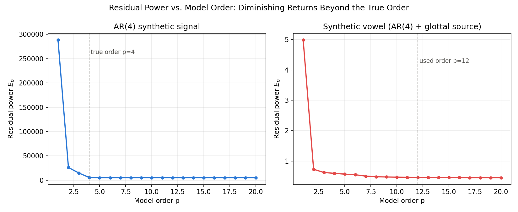
Residual power vs. model order for the AR(4) signal and the synthetic vowel

The left panel (AR(4) signal) flattens almost completely past \(p=4\) ; the right panel (synthetic vowel) likewise flattens near the \(p=12\) used in practice. Pushing the order higher barely reduces \(E_p\) further, while the risk of overfitting (tracking glottal harmonics) keeps growing — so this “elbow” location is a practical guide for choosing the model order.

LPC Spectral Envelope

A canonical LPC visualization overlays the magnitude response of the all-pole filter \(H(z) = 1/A(z)\) (the LPC spectrum) on the raw signal spectrum. The LPC spectrum smoothly tracks the envelope of the raw spectrum while ignoring the harmonic fine structure.

import numpy as np
import matplotlib.pyplot as plt
from scipy.signal import lfilter, freqz


def synth_vowel(fs=8000, duration=0.04, f0=140, ar=None, noise=0.02, seed=0):
    """Synthetic vowel: glottal pulse train through an AR vocal-tract filter."""
    np.random.seed(seed)
    t = np.arange(0, duration, 1 / fs)
    glottal = np.zeros_like(t)
    period = int(fs / f0)
    for k in range(0, len(t), period):
        L = min(30, len(t) - k)
        glottal[k : k + L] = np.exp(-np.arange(L) * 0.15)
    voice = lfilter([1.0], ar, glottal)
    voice = voice / (np.max(np.abs(voice)) + 1e-8)
    voice += noise * np.random.randn(len(voice))
    return t, voice


# Vowel "a"-like AR(4): formants F1≈800, F2≈1200 Hz (roots of A(z) are inside the unit circle: stable)
fs = 8000
ar_true = [1.0, -2.6895, 3.6076, -2.4801, 0.8546]
t, voice = synth_vowel(fs=fs, duration=0.04, f0=140, ar=ar_true, noise=0.02)

# LPC estimation (windowed to reduce spectral leakage)
window = np.hamming(len(voice))
a_est, E, _ = lpc(voice * window, p=12)
A = np.concatenate(([1.0], a_est))   # A(z) = 1 + a_1 z^-1 + ... + a_p z^-p
print("Estimated LPC coefficients (p=12):", a_est)
print("Residual power E:", E)

# Raw spectrum
n_fft = 1024
X = np.fft.rfft(voice * window, n=n_fft)
freqs = np.fft.rfftfreq(n_fft, d=1 / fs)
log_spec = 20 * np.log10(np.abs(X) + 1e-10)

# LPC spectrum: H(e^{jw}) = sqrt(E) / A(e^{jw})
w, H = freqz([np.sqrt(E)], A, worN=n_fft // 2 + 1, fs=fs)
lpc_spec_db = 20 * np.log10(np.abs(H) + 1e-10)

fig, ax = plt.subplots(figsize=(11, 5))
ax.plot(freqs, log_spec, color="steelblue", alpha=0.6, label="Log spectrum (windowed)")
ax.plot(w, lpc_spec_db, color="red", linewidth=2, label="LPC envelope (p=12)")
ax.set_ylim(-40, 40)
ax.axvline(820.5, color="gray", linestyle=":", linewidth=1)
ax.text(835, 35, "F1", color="gray", fontsize=10)
ax.axvline(1197.5, color="gray", linestyle=":", linewidth=1)
ax.text(1212, 35, "F2", color="gray", fontsize=10)
ax.set_xlabel("Frequency [Hz]")
ax.set_ylabel("Magnitude [dB]")
ax.set_title("LPC Spectral Envelope vs. Raw Spectrum")
ax.set_xlim(0, fs / 2)
ax.legend()
ax.grid(True, alpha=0.3)
plt.tight_layout()
plt.savefig("lpc_spectral_envelope.png", dpi=150, bbox_inches="tight")
plt.show()

Estimated LPC coefficients (p=12): [-1.7831  0.9418  0.4716 -0.2637 -0.4911  0.2977  0.022   0.1982 -0.252
 -0.1395  0.2205 -0.0617]
Residual power E: 0.4598260612610578

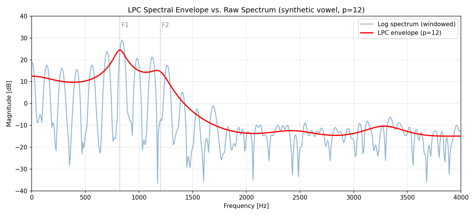
LPC spectral envelope overlaid on the raw log spectrum of a synthetic vowel, showing formants F1 and F2

The figure shows the finely-ripple raw spectrum (blue, glottal harmonics at regular spacing) against the LPC spectrum (red, \(p=12\) ), which smoothly traces only two resonance peaks (F1 \(\approx 820\) Hz, F2 \(\approx 1198\) Hz — computed exactly in the next section). The glottal harmonic ripple is entirely ignored, leaving only the low-order envelope structure corresponding to vocal-tract resonances.

Formant Estimation

Formants correspond to the roots (poles) of \(A(z)\) . For a pole \(z = r e^{j\theta}\) with \(r\) close to the unit circle, the resonance has

\[F = \frac{\theta}{2\pi}\, f_s,\qquad \mathrm{BW} = -\frac{\ln r}{\pi}\, f_s. \tag{17}\]

import numpy as np


def lpc_formants(a, fs, max_bw=400.0, min_freq=90.0):
    """
    Extract formant frequencies and bandwidths from LPC coefficients.

    Parameters
    ----------
    a : np.ndarray
        LPC coefficients [a_1, ..., a_p] (a_0 = 1 not included).
    fs : float
        Sampling frequency [Hz].
    max_bw : float
        Maximum bandwidth [Hz] for a pole to be counted as a formant.
    min_freq : float
        Minimum frequency [Hz] for a pole to be counted as a formant.

    Returns
    -------
    formants : list of (freq_Hz, bandwidth_Hz)
    """
    A = np.concatenate(([1.0], a))
    roots = np.roots(A)
    # Keep only roots in the upper half-plane (avoid conjugate duplicates)
    roots = roots[np.imag(roots) > 0]

    formants = []
    for r in roots:
        theta = np.arctan2(np.imag(r), np.real(r))
        magnitude = np.abs(r)
        f = theta / (2 * np.pi) * fs
        bw = -np.log(max(magnitude, 1e-10)) / np.pi * fs
        if f >= min_freq and bw <= max_bw:
            formants.append((f, bw))

    return sorted(formants, key=lambda x: x[0])


formants = lpc_formants(a_est, fs)
for i, (f, bw) in enumerate(formants[:4], start=1):
    print(f"F{i}: {f:7.1f} Hz   (BW = {bw:5.1f} Hz)")

F1:   820.5 Hz   (BW =  98.1 Hz)
F2:  1197.5 Hz   (BW = 164.6 Hz)

Only two formants from the \(p=12\) model satisfy the min_freq=90, max_bw=400 criteria (higher-order poles are rejected for having too wide a bandwidth). The design-time ground truth — computed directly from the roots of the order-4 ar_true polynomial — is F1 \(= 799.9\) Hz (BW \(= 80.0\) Hz), F2 \(= 1200.0\) Hz (BW \(= 120.1\) Hz). The errors against the \(p=12\) estimate are \(+20.6\) Hz for F1 and \(-2.5\) Hz for F2, which is a good recovery given the short 320-sample frame and additive noise. The lower formants F1 and F2 are the dominant perceptual cues for vowel identity, and the classical F1-F2 plane is widely used to separate vowels.

Relation to the Cepstrum: LPC Cepstrum

There is a direct recursion (Schroeder’s formula) that converts LPC coefficients to cepstral coefficients \(c[m]\) . With \(a_0 = 1\) ,

\[c[1] = -a_1, \tag{18}\] \[c[m] = -a_m - \sum_{k=1}^{m-1} \frac{k}{m}\, c[k]\, a_{m-k}, \qquad m = 2, 3, \ldots \tag{19}\]

LPC cepstral coefficients are linear in the log-spectral domain, which makes distance computations stable, and they have long been used as features for speech and speaker recognition. Compared to the FFT-based cepstrum (see Cepstrum Analysis: Theory and Python Implementation ), the LPC cepstrum gives a smoother representation of the low-quefrency (vocal-tract) region.

import numpy as np


def lpc_to_cepstrum(a, n_cep):
    """
    Convert LPC coefficients [a_1, ..., a_p] to LPC cepstrum c[1..n_cep].
    """
    p = len(a)
    c = np.zeros(n_cep)
    for m in range(1, n_cep + 1):
        if m <= p:
            c[m - 1] = -a[m - 1]
        # Recursive term
        s = 0.0
        for k_ in range(1, m):
            if (m - k_) <= p:
                s += (k_ / m) * c[k_ - 1] * a[m - k_ - 1]
        c[m - 1] -= s
    return c


cep = lpc_to_cepstrum(a_est, n_cep=20)
print("LPC cepstrum c[1..10]:", cep[:10])

LPC cepstrum c[1..10]: [ 1.78314  0.64802 -0.26099 -0.60069 -0.24648 -0.02235  0.25715  0.11109
  0.06295  0.1004 ]

Starting from \(c[1] = -a_1 = 1.7831\) (matching Eq. (18)), the coefficients decay in amplitude as the order increases — the typical shape for a well-behaved LPC cepstrum. The negative peaks around \(c[3]\) and \(c[4]\) reflect the spectral-envelope shape imposed by the F1/F2 formant structure.

Practical Considerations

Item	Recommendation
Sampling frequency	8 kHz (telephone band) or 16 kHz (wideband speech)
Model order \(p\)	\(p \approx f_s/1000 + 2 \text{ to } 4\) (10–12 at 8 kHz)
Frame length	20–30 ms (within which stationarity is approximately valid)
Window	Hamming / Hanning (suppresses spurious poles from edge jumps)
Pre-emphasis	\(y[n] = x[n] - 0.95\, x[n-1]\) (flattens spectral tilt)
Stability	\(\lvert k_m \rvert < 1\) from Levinson-Durbin guarantees stable \(1/A(z)\)
Excessive order	Tracks glottal harmonics → spurious formants
Non-stationary intervals	Plosives and boundaries → re-segment frames
Hand-picked AR truth	A hand-picked “true” AR polynomial is not automatically stable — check its roots lie inside the unit circle

Pre-emphasis is especially important: it compensates the roughly \(-12\) dB/octave glottal source tilt, prevents the poles from being biased toward low frequencies, and improves the accuracy of formant bandwidth estimates.

Modern Developments: LPC Meets Neural Vocoders

The all-pole filter established half a century ago is still used today as an efficient inductive bias inside neural speech synthesis. FARGAN (Framewise Autoregressive GAN) by Valin, Mustafa, & Büthe (2024, IEEE Signal Processing Letters, vol. 31, pp. 2115-2119) is the successor to the neural vocoder LPCNet: it combines linear-prediction-based pitch prediction with subframe-wise autoregressive generation inside a GAN framework, achieving better quality than existing low-complexity vocoders at only 600 MFLOPS. This is a clear example of the core LPC idea — predicting the current sample from a linear combination of past samples — surviving the transition from a purely statistical model to an inductive bias inside a neural network.

Summary

The linear-prediction model predicts the current sample from a linear combination of \(p\) past samples; it is an all-pole AR model whose residual is whitened.
Minimizing the sum of squared residuals leads to the normal equations, which in autocorrelation form become the Yule-Walker equations with a symmetric Toeplitz matrix.
The Levinson-Durbin algorithm updates coefficients order by order through the reflection coefficient \(k_m\) , solving the system in \(O(p^2)\) .
Reflection coefficients always satisfy \(|k_m| < 1\) , and they correspond physically to boundary reflection ratios in an acoustic-tube model of the vocal tract.
The LPC spectrum \(1/|A(e^{j\omega})|\) captures the spectral envelope while ignoring glottal harmonics, and the poles of \(A(z)\) correspond to formants.
Schroeder’s recursion converts LPC coefficients into the LPC cepstrum, a long-standing feature for speech and speaker recognition.
In practice, pre-emphasis, an appropriate window, and the rule of thumb \(p \approx f_s/1000 + 2 \text{ to } 4\) for the model order are decisive for quality, and empirically the residual-power reduction rate drops by more than an order of magnitude right at the true order.
Hand-picked AR coefficients are not automatically stable — always verify with np.roots that the roots of \(A(z)\) lie inside the unit circle.
The all-pole idea behind LPC remains in active use as an inductive bias inside neural vocoders such as FARGAN (2024).

Autocorrelation and Cross-Correlation: Theory and Python Implementation — defines the autocorrelation that fills both sides of the Yule-Walker equations and presents the FFT-based fast computation.
Cepstrum Analysis: Theory and Python Implementation — the FFT-based cepstrum that complements the LPC cepstrum from Schroeder’s recursion.
Fast Fourier Transform (FFT): Mechanism and Python Implementation — the FFT/DFT used to visualize LPC spectral envelopes and to compute autocorrelation efficiently.
Window Functions and Power Spectral Density (PSD): Theory and Python Implementation — windowing that precedes LPC estimation and PSD estimation via Welch’s method.
Wiener Filter: Theory and Python Implementation — another classical least-squares-derived linear filter, closely related to the LPC formulation.
Time-Series Forecasting with ARIMA Models — applications of the same AR family from the time-series forecasting side.

References

Atal, B. S., & Hanauer, S. L. (1971). “Speech analysis and synthesis by linear prediction of the speech wave.” Journal of the Acoustical Society of America, 50(2B), 637-655.
Itakura, F., & Saito, S. (1968). “Analysis synthesis telephony based on the maximum likelihood method.” Proceedings of the 6th International Congress on Acoustics, C-17-20.
Makhoul, J. (1975). “Linear prediction: A tutorial review.” Proceedings of the IEEE, 63(4), 561-580.
Markel, J. D., & Gray, A. H. (1976). Linear Prediction of Speech. Springer-Verlag.
Rabiner, L. R., & Schafer, R. W. (2010). Theory and Applications of Digital Speech Processing. Pearson.
Valin, J.-M., Mustafa, A., & Büthe, J. (2024). “Very Low Complexity Speech Synthesis Using Framewise Autoregressive GAN (FARGAN) with Pitch Prediction.” IEEE Signal Processing Letters, 31, 2115-2119. arXiv:2405.21069
SciPy linalg.solve_toeplitz documentation
Librosa: librosa.lpc