Introduction
A Bode plot visualizes the frequency response \(H(j\omega)\) of a linear time-invariant system as two stacked plots: magnitude [dB] and phase [degrees] on a logarithmic frequency axis. Systematized by Hendrik Bode in the 1930s for control engineering, it is now the standard tool for filter design, transfer function analysis, and stability evaluation across signal processing and control.
For filter design specifically, every key trait of Butterworth (maximally flat), Chebyshev (equiripple), highpass and lowpass (roll-off rate) is visible on a Bode plot. This article consolidates the math, reading techniques, and Python implementation so you can use the Bode plot as a cross-cutting hub for understanding all of these filters.
Mathematical Background
Transfer Function and Frequency Response
For a continuous-time LTI system with transfer function \(H(s)\) , the frequency response is obtained by substituting \(s = j\omega\) :
\[H(j\omega) = |H(j\omega)| \, e^{j\angle H(j\omega)} \tag{1}\]A Bode plot decomposes this complex-valued function into two plots:
- Magnitude plot: \(20\log_{10}|H(j\omega)|\) vs. \(\log_{10}\omega\)
- Phase plot: \(\angle H(j\omega)\) (degrees) vs. \(\log_{10}\omega\)
The Decibel Definition
Expressing magnitude in decibels turns multiplication into addition. For two systems \(H_1, H_2\) in series:
\[20\log_{10}|H_1 H_2| = 20\log_{10}|H_1| + 20\log_{10}|H_2| \tag{2}\]This means a Bode plot of a higher-order filter is the sum of the plots of its first-order factors, which makes complex filters tractable by superposition of simple shapes.
Phase Delay and Group Delay
Two key quantities readable from the phase plot are phase delay and group delay:
\[\tau_p(\omega) = -\frac{\angle H(j\omega)}{\omega}, \quad \tau_g(\omega) = -\frac{d\angle H(j\omega)}{d\omega} \tag{3}\]Group delay \(\tau_g\) is directly the slope of the phase plot and indicates waveform distortion. A linear-phase FIR filter has a constant group delay, which appears on a Bode plot as a phase that is a strictly linear function of frequency.
Bode Plots of 1st- and 2nd-Order Systems
First-Order Lowpass
\[H(s) = \frac{1}{1 + s/\omega_c} \tag{4}\]with magnitude
\[|H(j\omega)| = \frac{1}{\sqrt{1 + (\omega/\omega_c)^2}} \tag{5}\]reads asymptotically as
- \(\omega \ll \omega_c\) : \(|H|_{dB} \approx 0\) dB (passband)
- \(\omega = \omega_c\) : \(|H|_{dB} = -3\) dB (cutoff)
- \(\omega \gg \omega_c\) : \(|H|_{dB} \approx -20\log_{10}(\omega/\omega_c)\) dB (-20 dB/dec roll-off)
The phase passes through \(-45^\circ\) at \(\omega_c\) and asymptotes to \(-90^\circ\) . A first-order highpass is the mirror image: a \(+20\) dB/dec rise in the low band and a phase rotation from \(+90^\circ\) down to \(0^\circ\) .
Second-Order Resonance
For a second-order system
\[H(s) = \frac{\omega_n^2}{s^2 + 2\zeta\omega_n s + \omega_n^2} \tag{6}\]the magnitude exhibits a resonant peak when \(\zeta < 1/\sqrt{2}\) , with peak value
\[M_p = \frac{1}{2\zeta\sqrt{1-\zeta^2}} \tag{7}\]Smaller \(\zeta\) gives a sharper peak. The passband ripple of Chebyshev filters and both-band ripple of elliptic filters can be seen as the combined effect of multiple such second-order resonances. The high-frequency roll-off is -40 dB/dec, twice as steep as the first-order case.
Filter Types and Their Bode Plot Signatures
| Filter | Passband | Roll-off | Phase |
|---|---|---|---|
| Butterworth (order \(N\) ) | Maximally flat | \(-20N\) dB/dec | Relatively smooth |
| Chebyshev Type I | Equiripple | \(-20N\) dB/dec | Steep near band edge |
| Elliptic (Cauer) | Both-band ripple | Steepest | Steepest |
| Highpass | Flat for \(f > f_c\) | \(-20N\) /dec low | \(+90N^\circ \to 0^\circ\) |
| Bandpass | Flat inside band | \(\pm 20N\) /dec | \(0^\circ\) at center |
| Notch | Deep dip at \(f_0\) | Very steep | \(\pm 90^\circ\) flip at \(f_0\) |
The Bode plot thus serves as a visual dictionary of filter species: order \(N\) is read from the roll-off slope, attenuation type from the passband/stopband ripple shape, and phase distortion from the curvature of the phase plot.
Python Implementation
Standard Approach with scipy.signal.bode
scipy.signal.bode generates Bode plot data directly from a continuous-time transfer function.
import numpy as np
import matplotlib.pyplot as plt
from scipy import signal

# --- 1st-order lowpass: H(s) = 1 / (1 + s/wc) ---
wc = 2 * np.pi * 100        # Cutoff angular frequency [rad/s] (100 Hz)
num = [1.0]
den = [1.0 / wc, 1.0]
system = signal.TransferFunction(num, den)

# bode returns magnitude [dB] and phase [deg]
w, mag, phase = signal.bode(system, w=np.logspace(0, 4, 1000))
f = w / (2 * np.pi)         # Convert to Hz

fig, (ax1, ax2) = plt.subplots(2, 1, figsize=(10, 7), sharex=True)

ax1.semilogx(f, mag, linewidth=2)
ax1.axhline(-3, color='gray', linestyle=':', label='-3 dB')
ax1.axvline(wc / (2 * np.pi), color='r', linestyle='--', label=f'$f_c$ = {wc/(2*np.pi):.0f} Hz')
ax1.set_ylabel('Magnitude [dB]')
ax1.set_title('Bode Plot - 1st-order Lowpass')
ax1.grid(True, which='both', alpha=0.3)
ax1.legend()

ax2.semilogx(f, phase, linewidth=2, color='orange')
ax2.axvline(wc / (2 * np.pi), color='r', linestyle='--')
ax2.axhline(-45, color='gray', linestyle=':', label='-45°')
ax2.set_xlabel('Frequency [Hz]')
ax2.set_ylabel('Phase [degrees]')
ax2.grid(True, which='both', alpha=0.3)
ax2.legend()

plt.tight_layout()
plt.show()
Using semilogx is essential: a linear axis crushes the low-frequency structure, eliminating the Bode plot’s main strength of viewing multi-decade behavior at a glance.
IIR Digital Filters
For IIR digital filters such as
Butterworth
and
Chebyshev
, use scipy.signal.freqz instead.
import numpy as np
import matplotlib.pyplot as plt
from scipy import signal

fs = 1000.0           # Sampling frequency [Hz]
fc = 100.0            # Cutoff [Hz]
orders = [2, 4, 8]

fig, (ax1, ax2) = plt.subplots(2, 1, figsize=(10, 8), sharex=True)

for N in orders:
    sos = signal.butter(N, fc, btype='low', fs=fs, output='sos')
    w, h = signal.sosfreqz(sos, worN=4096, fs=fs)

    # Magnitude (log freq + dB)
    ax1.semilogx(w, 20 * np.log10(np.abs(h) + 1e-12), label=f'N={N}', linewidth=2)
    # Phase (unwrap to remove 360° jumps)
    ax2.semilogx(w, np.degrees(np.unwrap(np.angle(h))), label=f'N={N}', linewidth=2)

ax1.axhline(-3, color='gray', linestyle=':', label='-3 dB')
ax1.axvline(fc, color='r', linestyle='--', alpha=0.5)
ax1.set_ylabel('Magnitude [dB]')
ax1.set_title('Bode Plot - Butterworth Lowpass (digital)')
ax1.set_ylim(-100, 5)
ax1.grid(True, which='both', alpha=0.3)
ax1.legend()

ax2.axvline(fc, color='r', linestyle='--', alpha=0.5)
ax2.set_xlabel('Frequency [Hz]')
ax2.set_ylabel('Phase [degrees]')
ax2.set_xlim(1, fs / 2)
ax2.grid(True, which='both', alpha=0.3)
ax2.legend()

plt.tight_layout()
plt.show()
Each unit increase in order \(N\) steepens the high-frequency roll-off by 20 dB/dec and deepens the phase rotation by an additional \(-90^\circ\) . This is the best exercise to develop intuition for predicting filter characteristics from order alone.
Side-by-Side Comparison of Multiple Filters
Computing each filter manually lets us overlay their Bode plots for direct comparison.
import numpy as np
import matplotlib.pyplot as plt
from scipy import signal

fs = 1000.0
fc = 100.0
N = 4
f = np.logspace(0, np.log10(fs / 2), 2000)

fig, (ax1, ax2) = plt.subplots(2, 1, figsize=(10, 8), sharex=True)

filters = {
    'Butterworth':  signal.butter(N, fc, btype='low', fs=fs, output='ba'),
    'Chebyshev I':  signal.cheby1(N, 1.0, fc, btype='low', fs=fs, output='ba'),
    'Chebyshev II': signal.cheby2(N, 40.0, fc, btype='low', fs=fs, output='ba'),
    'Elliptic':     signal.ellip(N, 1.0, 40.0, fc, btype='low', fs=fs, output='ba'),
}

for name, (b, a) in filters.items():
    _, h = signal.freqz(b, a, worN=f, fs=fs)
    ax1.semilogx(f, 20 * np.log10(np.abs(h) + 1e-12), label=name, linewidth=2)
    ax2.semilogx(f, np.degrees(np.unwrap(np.angle(h))), label=name, linewidth=2)

ax1.axvline(fc, color='r', linestyle='--', alpha=0.5, label=f'$f_c$ = {fc} Hz')
ax1.axhline(-3, color='gray', linestyle=':', alpha=0.5)
ax1.set_ylabel('Magnitude [dB]')
ax1.set_title(f'Bode Plot Comparison (N={N})')
ax1.set_ylim(-80, 5)
ax1.grid(True, which='both', alpha=0.3)
ax1.legend()

ax2.set_xlabel('Frequency [Hz]')
ax2.set_ylabel('Phase [degrees]')
ax2.grid(True, which='both', alpha=0.3)
ax2.legend()

plt.tight_layout()
plt.savefig("bode_plot_comparison.png", dpi=150)
plt.show()
![Bode plot comparison of Butterworth, Chebyshev I, Chebyshev II, and elliptic filters (all 4th order, 100 Hz cutoff). Top: magnitude [dB]. Bottom: phase [deg]](/posts/20260521_bode_plot/bode_plot_comparison.png)
At identical order and cutoff, the Butterworth’s flat passband, Chebyshev I’s passband ripple, Chebyshev II’s stopband ripple, and the elliptic filter’s both-band ripple can be directly compared on the same Bode plot.
Design Guidelines
Choosing the Order from Cutoff Specifications
Given a passband edge \(f_p\) with maximum attenuation \(A_p\) [dB] and stopband edge \(f_s\) with minimum attenuation \(A_s\) [dB], the Butterworth order is
\[N \geq \frac{\log_{10}\!\left(\dfrac{10^{A_s/10} - 1}{10^{A_p/10} - 1}\right)}{2\log_{10}(f_s / f_p)} \tag{8}\]which is essentially “from two points on the Bode plot, infer the slope and back out the required roll-off rate.” scipy.signal.buttord automates this.
Numerical example: requiring at most \(A_p = 1\)
dB attenuation at \(f_p = 80\)
Hz and at least \(A_s = 40\)
dB attenuation at \(f_s = 150\)
Hz, hand-evaluating Eq. (8) gives \(N \geq 8.40\)
, rounded up to \(N=9\)
. Running scipy.signal.buttord(80, 150, 1.0, 40.0, analog=True) also returns \(N=9\)
(\(\omega_n=86.24\)
), matching the closed-form calculation exactly. Switching to analog=False (a digital filter with \(f_s=1000\)
Hz using the bilinear transform) for the same specs drops the required order to \(N=8\)
: the bilinear transform’s frequency warping effectively widens the transition band at higher frequencies, so applying the analog formula (Eq. 8) directly to a digital filter design can overestimate the required order.
Watch the Phase
A steeper magnitude roll-off comes at the cost of stronger phase rotation and more frequency-dependent group delay:
- Audio and medical signals (avoid phase distortion): use
FIR for linear phase
, or apply
filtfiltfor zero-phase processing - Real-time control (minimize group delay): Bessel filter or low-order Butterworth
- Passband flatness is top priority: Butterworth
- Sharpest transition is top priority: Chebyshev or elliptic
The phase plot of a Bode diagram captures this magnitude/phase trade-off at a single glance.
Relation to Adaptive Filters
Bode plots only make sense for time-invariant fixed filters. Adaptive filters such as LMS/RLS have coefficients that vary over time, so a Bode plot is only a snapshot of one instant. Conversely, the Bode plot of a target response can be the goal that an adaptive filter learns to approximate.
Connection to FFT and PSD
A Bode plot describes the filter itself. To see how a real signal behaves after passing through it, combine the filter with FFT and windowing + PSD estimation . From input spectrum \(X(f)\) and output spectrum \(Y(f) = H(f) X(f)\) , estimating \(|H(f)| = |Y(f)/X(f)|\) gives an empirical Bode plot, which is the fundamental principle of system identification.
Pole/Zero Roll-off: A Rigorous Derivation of the Asymptotes
So far we have only stated the results — “it becomes \(-20\) dB/dec,” “the phase passes through \(-45°\) ” — without deriving them. Here we derive them directly from algebra, and numerically verify that multiple poles and zeros really do superpose by simple addition.
Why a Single Real Pole Produces Exactly -20 dB/dec
Converting the magnitude of Eq. (5), \(|H(j\omega)| = 1/\sqrt{1+(\omega/\omega_c)^2}\) , to decibels gives
\[ |H(j\omega)|_{dB} = -20\log_{10}\sqrt{1+(\omega/\omega_c)^2} = -10\log_{10}\!\left[1+\left(\frac{\omega}{\omega_c}\right)^{2}\right] \]At high frequency \(\omega \gg \omega_c\) , the \(1\) inside the brackets becomes negligible, so
\[ |H(j\omega)|_{dB} \ \xrightarrow{\ \omega \gg \omega_c\ }\ -20\log_{10}\!\left(\frac{\omega}{\omega_c}\right) \tag{9} \]which is a linear function of \(\log_{10}\omega\) . Computing the change when \(\omega\) increases tenfold (one decade):
\[ -20\log_{10}\!\left(\frac{10\omega}{\omega_c}\right) - \left[-20\log_{10}\!\left(\frac{\omega}{\omega_c}\right)\right] = -20\log_{10}10 = -20\ \text{dB} \tag{10} \]This shows the magnitude drops by exactly 20 dB for every decade increase in frequency, derived from algebra alone. This is not an approximation — it is the exact slope of the asymptote in the limit \(\omega \gg \omega_c\) .
The phase is \(\angle H(j\omega) = -\arctan(\omega/\omega_c)\) , which passes through exactly \(-45°\) at \(\omega=\omega_c\) (since \(\arctan 1 = 45°\) ) and asymptotes to \(-90°\) as \(\omega\to\infty\) . How far does the textbook straight-line approximation ("\(0°\) at \(0.1\omega_c\) , \(-90°\) at \(10\omega_c\) , linear in between") deviate from the true arctangent curve? Let’s check numerically.
import numpy as np
from scipy import signal

wc = 10.0
sys_pole = signal.TransferFunction([1.0], [1.0 / wc, 1.0])

for wt in [0.1 * wc, wc, 10 * wc]:
    _, mag, phase = signal.bode(sys_pole, w=np.array([wt]))
    print(f"w={wt:6.1f}: mag={mag[0]:7.3f} dB, phase={phase[0]:7.2f} deg")
Output:
w=   1.0: mag= -0.043 dB, phase=  -5.71 deg
w=  10.0: mag= -3.010 dB, phase= -45.00 deg
w= 100.0: mag=-20.043 dB, phase= -84.29 deg
The straight-line approximation predicts \(0°\) at \(0.1\omega_c\) and \(-90°\) at \(10\omega_c\) , but the actual values are \(-5.71°\) and \(-84.29°\) respectively — an error of exactly \(5.71°\) at each decade edge (\(=\arctan(0.1)\times180/\pi\) ). At \(\omega_c\) itself, the approximation and the exact solution agree exactly at \(-45°\) .
A Zero Is the Mirror Image
A zero \(H(s) = 1+s/\omega_c\) has the numerator/denominator relationship of a pole reversed, so every sign in the argument above flips.
\[ |H(j\omega)|_{dB} \ \xrightarrow{\ \omega \gg \omega_c\ }\ +20\log_{10}\!\left(\frac{\omega}{\omega_c}\right) \tag{11} \]The phase is \(+\arctan(\omega/\omega_c)\) , increasing monotonically from \(0°\) to \(+90°\) . Where a pole gives “magnitude down 20 dB/dec, phase \(0°\) to \(-90°\) ,” a zero gives “magnitude up 20 dB/dec, phase \(0°\) to \(+90°\) ” — both magnitude and phase are mirrored.
Multiple Poles and Zeros Simply Add on the Log Axis
The decibel additivity of Eq. (2) holds regardless of how many poles or zeros there are: the magnitude of a cascaded system should be the simple sum of each element’s dB value. Let’s verify this numerically.
import numpy as np
from scipy import signal

wc1, wc2, wcz = 5.0, 50.0, 500.0
sys1 = signal.TransferFunction([1.0], [1.0 / wc1, 1.0])   # pole (wc1 = 5 rad/s)
sys2 = signal.TransferFunction([1.0], [1.0 / wc2, 1.0])   # pole (wc2 = 50 rad/s)
sysz = signal.TransferFunction([1.0 / wcz, 1.0], [1.0])   # zero (wcz = 500 rad/s)

num_casc = np.polymul([1.0 / wcz, 1.0], [1.0])
den_casc = np.polymul([1.0 / wc1, 1.0], [1.0 / wc2, 1.0])
sys_casc = signal.TransferFunction(num_casc, den_casc)     # full cascade: 2 poles + 1 zero

w = np.array([1000.0])
_, mag1, _ = signal.bode(sys1, w=w)
_, mag2, _ = signal.bode(sys2, w=w)
_, magz, _ = signal.bode(sysz, w=w)
_, mag_casc, _ = signal.bode(sys_casc, w=w)

print(f"pole1={mag1[0]:.4f} dB, pole2={mag2[0]:.4f} dB, zero={magz[0]:.4f} dB")
print(f"sum of individual dB = {mag1[0] + mag2[0] + magz[0]:.4f} dB")
print(f"cascade actual dB    = {mag_casc[0]:.4f} dB")
Output (\(\omega=1000\) rad/s):
pole1=-46.0207 dB, pole2=-26.0314 dB, zero=6.9897 dB
sum of individual dB = -65.0625 dB
cascade actual dB    = -65.0625 dB
The sum of the individual dB values, \(-65.0625\) dB, matches the directly-computed cascade transfer function to 4 decimal places. The fact that this two-pole-one-zero system (net relative degree 1) converges to the roll-off of a single first-order pole (\(-20\) dB/dec) is directly readable from this addition.
Advanced Topics: Non-Minimum-Phase Systems and Gain/Phase Margins
So far the focus has been “how to read the Bode plot of a given transfer function.” Now we turn to three pitfalls that are easy to miss when using Bode plots for control-system stability analysis, verifying each numerically with scipy.signal.
Non-Minimum-Phase Systems (RHP Zero): Identical Magnitude, Very Different Phase
A system with a zero in the left half-plane (LHP, \(\mathrm{Re}(s)<0\) ) is called minimum phase; one with a zero in the right half-plane (RHP, \(\mathrm{Re}(s)>0\) ) is non-minimum phase. For the same pole locations, moving a zero from the LHP to the RHP leaves the magnitude \(|H(j\omega)|\) completely unchanged. A zero at \(s=-a\) (LHP) gives \(|-a+j\omega|=\sqrt{a^2+\omega^2}\) ; a zero at \(s=+a\) (RHP) gives \(|a-j\omega|=\sqrt{a^2+\omega^2}\) — the absolute values are identical by construction.
\[ H_{\mathrm{mp}}(s) = \frac{s+1}{(s+2)(s+5)}, \qquad H_{\mathrm{nmp}}(s) = \frac{-s+1}{(s+2)(s+5)} \tag{12} \](\(H_{\mathrm{mp}}\) is minimum phase with a zero at \(s=-1\) ; \(H_{\mathrm{nmp}}\) is non-minimum phase with a zero at \(s=+1\) . Both share the same poles.)
import numpy as np
from scipy import signal

num_mp = [1, 1]     # zero at s=-1 (LHP)
num_nmp = [-1, 1]   # zero at s=+1 (RHP)
den = [1, 7, 10]    # (s+2)(s+5)

sys_mp = signal.TransferFunction(num_mp, den)
sys_nmp = signal.TransferFunction(num_nmp, den)

w = np.logspace(-2, 2, 2000)
w, mag_mp, phase_mp = signal.bode(sys_mp, w=w)
_, mag_nmp, phase_nmp = signal.bode(sys_nmp, w=w)

print("max|mag_mp - mag_nmp| =", np.max(np.abs(mag_mp - mag_nmp)))
print(f"phase_mp(w=100)  = {phase_mp[-1]:.2f} deg")
print(f"phase_nmp(w=100) = {phase_nmp[-1]:.2f} deg")
Output:
max|mag_mp - mag_nmp| = 7.105427357601002e-15
phase_mp(w=100)  = -86.56 deg
phase_nmp(w=100) = -265.42 deg
The magnitude difference is at floating-point noise level (\(7\times10^{-15}\) ) — effectively identical. The phase, however, differs enormously: at \(\omega=100\) rad/s the minimum-phase system is at \(-86.56°\) (asymptoting to \(-90°\) , matching relative degree 1), while the non-minimum-phase system is at \(-265.42°\) (asymptoting to \(-270°\) ) — a gap of nearly \(180°\) . The RHP zero adds an extra \(-180°\) of phase lag at high frequency compared to the LHP zero (twice the phase rotation).
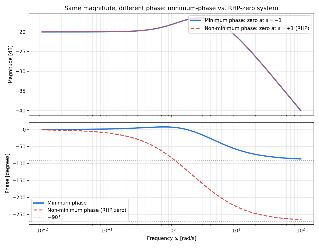
Why this matters in practice: in feedback control, a non-minimum-phase zero imposes the constraint that the control bandwidth must stay well below the zero frequency, or the closed loop tends to destabilize. Since the magnitude plot alone cannot distinguish it from a minimum-phase system, always check the phase plot — this is the golden rule for catching non-minimum-phase behavior. Inverted pendulums and aircraft pitch control (the momentary reverse motion right after a control input) are classic examples.
Gain Margin vs. Phase Margin: Two Different Stability Indicators
For an open-loop transfer function \(L(j\omega)\) , the stability margin is defined as two independent quantities:
\[ \mathrm{PM} = 180° + \angle L(j\omega_{gc}), \quad \text{where}\ |L(j\omega_{gc})| = 0\ \mathrm{dB} \] \[ \mathrm{GM} = -20\log_{10}|L(j\omega_{pc})|, \quad \text{where}\ \angle L(j\omega_{pc}) = -180° \]Here \(\omega_{gc}\) is the gain-crossover frequency (where the magnitude crosses 0 dB) and \(\omega_{pc}\) is the phase-crossover frequency (where the phase crosses \(-180°\) ). These are independent indicators evaluated at different frequencies by definition — one can be large while the other is small.
Let’s verify this numerically for a third-order open-loop system \(L(s)=K/[s(s+1)(s+5)]\) (one integrator plus two real poles) with \(K=8\) .
import numpy as np
from scipy import signal


def find_margins(num, den, w):
    sys = signal.TransferFunction(num, den)
    w, mag, phase = signal.bode(sys, w=w)

    gc_idx = np.where(np.diff(np.sign(mag)))[0][0]
    w0, w1 = w[gc_idx], w[gc_idx + 1]
    m0, m1 = mag[gc_idx], mag[gc_idx + 1]
    wgc = w0 + (0 - m0) * (w1 - w0) / (m1 - m0)
    p0, p1 = phase[gc_idx], phase[gc_idx + 1]
    pm = 180 + (p0 + (wgc - w0) * (p1 - p0) / (w1 - w0))

    pc_idx = np.where(np.diff(np.sign(phase + 180)))[0][0]
    w0, w1 = w[pc_idx], w[pc_idx + 1]
    p0, p1 = phase[pc_idx], phase[pc_idx + 1]
    wpc = w0 + (-180 - p0) * (w1 - w0) / (p1 - p0)
    m0, m1 = mag[pc_idx], mag[pc_idx + 1]
    gm = -(m0 + (wpc - w0) * (m1 - m0) / (w1 - w0))
    return wgc, pm, wpc, gm


K = 8.0
den = np.polymul([1, 0], np.polymul([1, 1], [1, 5]))
w = np.logspace(-2, 2, 400000)
wgc, pm, wpc, gm = find_margins([K], den, w)
print(f"wgc={wgc:.4f} rad/s, PM={pm:.2f} deg")
print(f"wpc={wpc:.4f} rad/s, GM={gm:.2f} dB")
Output:
wgc=1.0689 rad/s, PM=31.02 deg
wpc=2.2361 rad/s, GM=11.48 dB
A common rule of thumb in practice is “\(\mathrm{GM}>6\) dB and \(\mathrm{PM}>45°\) .” This system has GM=11.48 dB, comfortably clearing the guideline, yet PM=31.02° falls short of the 45° guideline — a level at which step-response overshoot and oscillation become noticeable. Looking only at the gain margin and concluding “we’re fine, it’s above 6 dB” would miss the transient-response degradation that the phase margin reveals.
![Bode plot of L(s)=8/[s(s+1)(s+5)]. Gain margin of 11.48 dB clears the guideline, but phase margin of 31.02° falls short of the 45° guideline](/posts/20260521_bode_plot/gain_phase_margin_bode.png)
In practice, always report both GM and PM together rather than judging stability margin from either alone. Systems with resonant peaks or higher order can even have multiple gain crossovers (“conditionally stable” systems), where the simple GM/PM definitions themselves break down (see Nyquist Plot and Root Locus for the more advanced treatment). This same GM/PM pairing is essential when tuning PID controller gains.
Resonant Peak and Damping Ratio \(\zeta\) : Numerically Verifying the \(M_p\) Formula
Let’s numerically verify the resonant peak formula from Eq. (7), \(M_p = 1/(2\zeta\sqrt{1-\zeta^2})\) (valid for \(\zeta<1/\sqrt2\approx0.7071\) ), across several values of \(\zeta\) .
import numpy as np
from scipy import signal

wn = 1.0
zetas = [0.05, 0.1, 0.2, 0.3, 0.5, 0.6, 1 / np.sqrt(2), 0.8, 1.0]

for zeta in zetas:
    num = [wn ** 2]
    den = [1, 2 * zeta * wn, wn ** 2]
    sys = signal.TransferFunction(num, den)
    w = np.logspace(-2, 1, 200000)
    w, mag, phase = signal.bode(sys, w=w)
    idx = np.argmax(mag)

    if zeta < 1 / np.sqrt(2):
        Mp_db_theory = 20 * np.log10(1 / (2 * zeta * np.sqrt(1 - zeta ** 2)))
    else:
        Mp_db_theory = 0.0  # no resonant peak for zeta >= 1/sqrt(2)
    print(f"zeta={zeta:.4f}: Mp_theory={Mp_db_theory:8.4f} dB, Mp_numeric={mag[idx]:8.4f} dB")
Output:
zeta=0.0500: Mp_theory= 20.0109 dB, Mp_numeric= 20.0109 dB
zeta=0.1000: Mp_theory= 14.0230 dB, Mp_numeric= 14.0230 dB
zeta=0.2000: Mp_theory=  8.1361 dB, Mp_numeric=  8.1361 dB
zeta=0.3000: Mp_theory=  4.8466 dB, Mp_numeric=  4.8466 dB
zeta=0.5000: Mp_theory=  1.2494 dB, Mp_numeric=  1.2494 dB
zeta=0.6000: Mp_theory=  0.3546 dB, Mp_numeric=  0.3546 dB
zeta=0.7071: Mp_theory=  0.0000 dB, Mp_numeric= -0.0000 dB
zeta=0.8000: Mp_theory=  0.0000 dB, Mp_numeric= -0.0002 dB
zeta=1.0000: Mp_theory=  0.0000 dB, Mp_numeric= -0.0009 dB
For \(\zeta<1/\sqrt2\) , theory and numerics agree to 4 decimal places. Past \(\zeta=1/\sqrt2\approx0.7071\) the resonant peak disappears (\(M_p=1=0\) dB), and for larger \(\zeta\) the magnitude decreases monotonically with no resonance (the slightly negative “numeric” values at \(\zeta=0.8, 1.0\) are a harmless numerical artifact of the peak-free curve’s maximum sitting essentially at the 0 dB point within the search window — not a contradiction of theory). Smaller \(\zeta\) gives a sharper, taller peak: at \(\zeta=0.05\) the peak reaches a full \(20\) dB (10x in voltage ratio).
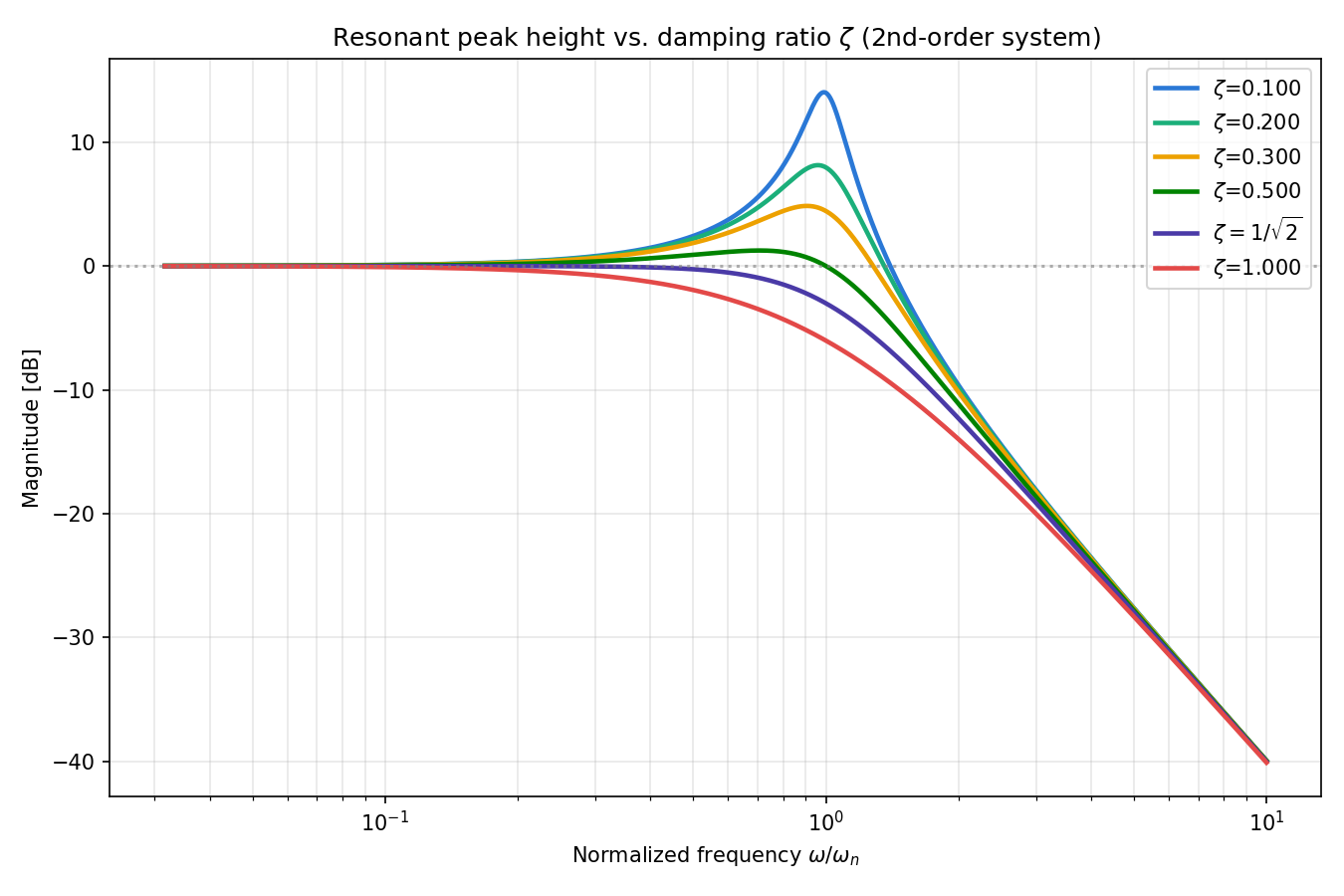
The passband ripple of Chebyshev filters and the both-band ripple of elliptic filters can be seen as the combined effect of multiple such resonant peaks. The fact that cascades of lightly-damped second-order sections trade stopband rejection for passband peaking (ripple) is, at its root, exactly this \(M_p\) formula at work.
Recent Research
Bode-plot-based frequency-domain analysis is a classical technique, but it remains an active research area even as data-driven and model-free control approaches gain prominence.
- Isoshima, Tanemura, & Chida (2023) proposed a method to estimate lower bounds on gain margin and phase margin purely from input-output data, without a model. Where classical Bode-plot analysis is model-based, this gives a stability-margin guarantee from measured frequency-response data alone.
- Ren, Quan, Xu, Wang, & Cai (2024) proposed a data-driven framework for defining and estimating stability margins for multi-input multi-output (MIMO) systems. Since SISO-style GM/PM does not directly carry over to MIMO systems, they systematize an experimental way to obtain stability margins from frequency-domain data.
- Broens, Butler, & Tóth (2024) proposed auto-tuning structured linear-parameter-varying (LPV) controllers based on frequency response function (FRF) estimates, applied to high-precision motion control in positioning systems — pointing toward automated Bode-plot reading and loop-shaping.
All three bridge the classical representation of Bode plots and frequency response with the modern demands of data-driven control and automation, showing that the magnitude/phase fundamentals derived in this article remain the bedrock of current control research.
Summary
- A Bode plot shows the frequency response \(H(j\omega)\) as magnitude [dB] + phase [deg] on a log frequency axis
- Decibels convert serial cascading into addition; the log axis makes multi-decade behavior uniformly readable
- A first-order pole/zero gives \(\pm 20\) dB/dec, a second-order resonance gives \(\pm 40\) dB/dec, and an \(N\) -th order filter gives \(\pm 20N\) dB/dec — an exact result derived from the asymptote of a linear function of \(\log_{10}\omega\) , confirmed numerically (algebraic identity, cascade additivity matching to 4 decimal places)
- The unique signatures of Butterworth, Chebyshev, elliptic, highpass, bandpass, and notch filters all appear directly on a Bode plot
- A non-minimum-phase system (RHP zero) has identical magnitude to its minimum-phase counterpart, yet its phase lags by nearly \(180°\) more at high frequency (verified numerically: \(-86.56°\) vs. \(-265.42°\) at \(\omega=100\) )
- Gain margin and phase margin are independent indicators evaluated at different frequencies — a real system exists with GM=11.48 dB (clearing the guideline) yet PM=31.02° (falling short) for \(L(s)=8/[s(s+1)(s+5)]\)
- The resonant peak \(M_p=1/(2\zeta\sqrt{1-\zeta^2})\) of a 2nd-order system (\(\zeta<1/\sqrt2\) ) matches theory and numerics to 4 decimal places, and grows sharper as \(\zeta\) shrinks
- In Python,
scipy.signal.bode(continuous-time) andscipy.signal.freqz(discrete-time) are the standard tools
See the related articles below for the design theory of each specific filter type.
Related Articles
- Nyquist Plot, Root Locus, and Stability Margins in Python - The follow-up that turns the phase and gain margins read from a Bode plot into closed-loop stability via the Nyquist plot and root locus — the direct continuation of this article for control-system design.
- PID Control: Fundamental Theory and the Role of Each Term - The gain margin / phase margin analysis in this article applies directly to evaluating the stability limits of PID gain tuning.
- PID Control in Python: Simulation and Tuning - See how the transient-response degradation from raising PID gains connects to the numerical GM/PM example here.
- H-infinity Control and Robust Stability: Theory and Python Implementation - Generalizes the classical frequency-domain indicators (Bode plot, GM/PM) covered here into a robust-control framework that explicitly handles uncertainty.
- Butterworth Filter Design: Theory and Python Implementation - The canonical IIR filter whose maximally flat roll-off is best understood on a Bode plot.
- Chebyshev Filter Design: Theory and Python Implementation - Learn how passband ripple appears on a Bode plot.
- Highpass Filter Design and Python Implementation - Read the low-frequency roll-off and \(+90^\circ\) phase rotation on a Bode plot.
- Lowpass Filter Design Compared - The most fundamental subject for Bode plot comparison.
- Bandpass Filter Design and Python Implementation - Observe band-centered magnitude and the symmetric phase profile.
- Notch Filter Design and Python Implementation - See the deep dip at \(f_0\) and the sharp phase flip in the Bode plot.
- FIR vs IIR Filters: Characteristics, Design, and Python Implementation - Understand how linear-phase FIR produces a straight-line phase plot.
- Adaptive Filters (LMS/RLS): Theory and Python Implementation - Time-varying filters that contrast with the time-invariant Bode plot.
- Fast Fourier Transform (FFT): Theory and Python Implementation - The FFT theory used to measure empirical Bode plots.
- Window Functions and PSD Estimation - Leakage suppression and PSD estimation for empirical Bode plots.
- Bessel Filter: Theory and Python Implementation - Bessel’s maximally flat group delay appears as a near-linear phase plot — the cleanest comparison target against Butterworth and Chebyshev phase responses.
- Time-Frequency Analysis Guide - Sister hub that extends from the time-invariant frequency response shown on a Bode plot to the FFT / STFT / wavelet / Hilbert toolkit for time-varying and non-stationary signals.
References
- Bode, H. W. (1945). Network Analysis and Feedback Amplifier Design. Van Nostrand.
- Ogata, K. (2010). Modern Control Engineering (5th ed.). Prentice Hall.
- Oppenheim, A. V., & Schafer, R. W. (2009). Discrete-Time Signal Processing (3rd ed.). Prentice Hall.
- Isoshima, K., Tanemura, M., & Chida, Y. (2023). “Data-driven estimation of the lower bounds of gain and phase margins”. Automatica, 153, 111008.
- Ren, J., Quan, Q., Xu, B., Wang, S., & Cai, K.-Y. (2024). “Data-driven stability margin for linear multivariable systems”. International Journal of Robust and Nonlinear Control, 34(13), 8844-8862.
- Broens, Y., Butler, H., & Tóth, R. (2024). “Frequency Domain Auto-tuning of Structured LPV Controllers for High-Precision Motion Control”. arXiv:2403.05878.
- scipy.signal.bode — SciPy documentation
- scipy.signal.freqz — SciPy documentation