Introduction
Monte Carlo optimization is a family of methods that minimize (or maximize) an objective \(f(x)\) using random sampling rather than gradients \(\nabla f\) . They shine exactly where gradient methods fail: non-differentiable objectives, black-box simulators, and multi-modal landscapes.
Cross-Entropy Method (CEM) , Simulated Annealing (SA) , Genetic Algorithms (GA) , MPPI , and Particle Swarm Optimization (PSO) are all canonical Monte Carlo optimizers built on the same “sample → evaluate → update” skeleton. This article positions each method side by side and organizes the shared framework, selection guidance, and Python implementation as a hub.
The Common Skeleton
Every Monte Carlo optimizer can be viewed as iterating three steps:
- Sample: draw \(N\) samples \(\{x^{(i)}\}_{i=1}^{N}\) from the current distribution \(p_t(x)\) or around the current solution \(x_t\)
- Evaluate: compute \(f(x^{(i)})\) for each sample
- Update: build the next distribution \(p_{t+1}\) or solution \(x_{t+1}\) from the evaluations
Symbolically the update is
\[ p_{t+1}(x) = \mathcal{U}\big(p_t,\, \{(x^{(i)}, f(x^{(i)}))\}_{i=1}^{N}\big) \tag{1} \]where \(\mathcal{U}\) is the method-specific update operator. CEM fits an empirical distribution to elite quantiles, SA accepts moves with Boltzmann probability, GA applies selection / crossover / mutation, MPPI computes a cost-exponentially-weighted average, and PSO updates velocities with inertia, cognitive, and social terms. All are different choices of the same \(\mathcal{U}\) .
Bayesian optimization is also a sampling-based optimizer, but it operates through a surrogate model (Gaussian process) and an acquisition function — it emphasizes “where to sample next” over “how to update a distribution.” Particle filters are a sibling family that uses Monte Carlo sampling for state estimation, with resampling mechanics mathematically equivalent to CEM’s elite selection and MPPI’s reweighting.
Method Comparison Table
| Method | Search strategy | Solution form | Typical use | Cost | Gradient |
|---|---|---|---|---|---|
| CEM | Distribution update (elite quantile) | Parametric distribution | Continuous opt, RL policy search | Medium (parallel-friendly) | Not needed |
| SA | Probabilistic acceptance (temperature) | Single solution | Combinatorial opt, TSP | Low (sequential) | Not needed |
| GA | Population evolution (crossover/mutation) | Population | Global opt, design problems | High (many evals) | Not needed |
| MPPI | Importance sampling (exp weights) | Distribution over trajectories | Model predictive control, robotics | Medium–high (needs parallelism) | Not needed |
| PSO | Inertia + cognitive + social | Swarm of particles | Continuous opt, swarm intelligence | Medium | Not needed |
| Bayesian optimization | Surrogate + acquisition | GP posterior | Expensive black-box problems | High (surrogate update) | Not needed (internal GP gradients) |
All methods share three properties: gradient-free, easy to parallelize, and robust to multi-modality. They differ in which probabilistic model they maintain and how the update concentrates mass on good regions.
Shared Python Framework
Each method fits the same skeleton; only sample and update change.
import numpy as np

def monte_carlo_optimize(
    f, sampler, updater, init_state, n_iter=50, n_samples=100, seed=0
):
    """
    Generic Monte Carlo optimization loop.

    Parameters
    ----------
    f          : callable  objective f(x) to minimize
    sampler    : callable  state -> array of shape (n_samples, dim)
    updater    : callable  (state, samples, scores) -> new state
    init_state : initial state (per-method distribution params, population, ...)
    n_iter     : number of iterations
    n_samples  : samples per iteration
    """
    rng = np.random.default_rng(seed)
    state = init_state
    history = []
    for t in range(n_iter):
        samples = sampler(state, n_samples, rng)
        scores = np.array([f(x) for x in samples])
        state = updater(state, samples, scores)
        best = scores.min()
        history.append(best)
    return state, np.array(history)


# === Example 1: CEM-style update (fit Gaussian to elite quantile) ===
def cem_sampler(state, n, rng):
    mu, sigma = state
    return rng.normal(mu, sigma, size=(n, mu.shape[0]))


def cem_updater(state, samples, scores, elite_frac=0.2):
    mu, sigma = state
    k = max(1, int(len(scores) * elite_frac))
    elite_idx = np.argsort(scores)[:k]
    elite = samples[elite_idx]
    return elite.mean(axis=0), elite.std(axis=0) + 1e-6


# === Example 2: PSO-style velocity update ===
def make_pso(dim, n_particles, w=0.7, c1=1.5, c2=1.5):
    def sampler(state, n, rng):
        x, v, pbest, pbest_val, gbest = state
        return x  # PSO evaluates the state itself

    def updater(state, samples, scores):
        x, v, pbest, pbest_val, gbest = state
        # personal best
        improved = scores < pbest_val
        pbest = np.where(improved[:, None], x, pbest)
        pbest_val = np.where(improved, scores, pbest_val)
        # global best
        g_idx = pbest_val.argmin()
        gbest = pbest[g_idx]
        # velocity / position update
        rng = np.random.default_rng()
        r1, r2 = rng.random(x.shape), rng.random(x.shape)
        v = w * v + c1 * r1 * (pbest - x) + c2 * r2 * (gbest - x)
        x = x + v
        return x, v, pbest, pbest_val, gbest

    return sampler, updater


# === Objective: Rastrigin (multi-modal benchmark) ===
def rastrigin(x, A=10.0):
    n = x.shape[0]
    return A * n + np.sum(x ** 2 - A * np.cos(2 * np.pi * x))


# === Optimize with CEM ===
dim = 5
init_state = (np.zeros(dim), np.ones(dim) * 2.0)
state, hist = monte_carlo_optimize(
    rastrigin, cem_sampler, cem_updater, init_state,
    n_iter=40, n_samples=200
)
print(f"CEM best: {hist.min():.4f}")
This skeleton ports to all of CEM / SA / GA / MPPI / PSO. For SA, sampler becomes a random walk around the current solution and updater applies the Metropolis acceptance rule. For GA, sampler returns the current population and updater does selection + crossover + mutation. For MPPI, sampler rolls out noisy control sequences and updater averages them with cost-exponential weights to refine the nominal control.
This generalization is also theoretically meaningful: CEM and MPPI share the same root in importance sampling with an optimal proposal distribution, as discussed in detail in the MPPI article .
Convergence Comparison Across All 5 Methods: A Verification Run
To test the “same skeleton, different \(\mathcal{U}\) ” claim directly, we ran CEM, SA, GA, MPPI, and PSO on the same benchmark, the same starting point, and the same evaluation budget, then compared the resulting convergence curves.
- Benchmark: a shifted 5-dimensional Rastrigin function. The global minimum sits at \(z = x - x^\ast = 0\) , shifted away from the origin (starting all methods at the origin would trivially favor whichever method happens to initialize its distribution there, hiding real differences)
- Starting point: all methods share
x0 = [-4, 4, -4, 4, -4], far from the optimum - Evaluation budget: 40 iterations × 200 samples/iteration = 8,000 total function evaluations for every method
- Randomness: the optimization loop itself is seeded with
np.random.default_rng(seed=0), and initial-population generation is seeded separately withnp.random.default_rng(seed=1), so the run is fully reproducible
We generalize updater to also receive the random generator rng (SA’s Metropolis acceptance and GA’s crossover/mutation both need randomness), extending the earlier signature from updater(state, samples, scores) to updater(state, samples, scores, rng).
import numpy as np

# --- shared benchmark: shifted Rastrigin (dim=5, global min 0 at x*=shift) ---
dim = 5
shift = np.array([3.0, -2.0, 1.0, -2.5, 4.0])


def rastrigin(x, A=10.0):
    z = x - shift
    n = z.shape[0]
    return A * n + np.sum(z**2 - A * np.cos(2 * np.pi * z))


x0 = np.array([-4.0, 4.0, -4.0, 4.0, -4.0])  # common starting point for every method


# --- generic loop (extended to also pass rng into updater) ---
def monte_carlo_optimize(f, sampler, updater, init_state, n_iter=40, n_samples=200, seed=0):
    rng = np.random.default_rng(seed)
    state = init_state
    history = []
    best_so_far = np.inf
    for t in range(n_iter):
        samples = sampler(state, n_samples, rng)
        scores = np.array([f(x) for x in samples])
        state = updater(state, samples, scores, rng)
        best_so_far = min(best_so_far, scores.min())
        history.append(best_so_far)
    return state, np.array(history)


# --- CEM: fit a Gaussian to the elite quantile ---
def cem_sampler(state, n, rng):
    mu, sigma = state
    return rng.normal(mu, sigma, size=(n, mu.shape[0]))


def cem_updater(state, samples, scores, rng, elite_frac=0.2):
    mu, sigma = state
    k = max(1, int(len(scores) * elite_frac))
    elite = samples[np.argsort(scores)[:k]]
    return elite.mean(axis=0), elite.std(axis=0) + 1e-6


# --- SA: draw n_samples proposals around the current solution, accept sequentially via Metropolis ---
def sa_sampler(state, n, rng, step=0.6):
    x, fx, T = state
    return x + rng.normal(0, step, size=(n, x.shape[0]))


def sa_updater(state, samples, scores, rng, cooling=0.93):
    x, fx, T = state
    for x_prop, f_prop in zip(samples, scores):
        if f_prop < fx or rng.random() < np.exp(-(f_prop - fx) / T):
            x, fx = x_prop, f_prop
    return x, fx, T * cooling


# --- GA: tournament selection + uniform crossover + mutation, 1-individual elitism ---
def ga_sampler(state, n, rng):
    return state  # the current population itself is the evaluation target


def ga_updater(state, samples, scores, rng, mutation_rate=0.2, mutation_scale=0.5, k=3):
    pop = samples
    n, d = pop.shape
    new_pop = np.empty_like(pop)
    for i in range(n):
        idx1 = rng.integers(0, n, size=k)
        p1 = pop[idx1[np.argmin(scores[idx1])]]
        idx2 = rng.integers(0, n, size=k)
        p2 = pop[idx2[np.argmin(scores[idx2])]]
        # uniform crossover (copy each gene from one parent; blend crossover shrinks
        # variance and converges prematurely on multi-modal functions, so we avoid it)
        cross_mask = rng.random(d) < 0.5
        child = np.where(cross_mask, p1, p2)
        mask = rng.random(d) < mutation_rate
        child = np.where(mask, child + rng.normal(0, mutation_scale, d), child)
        new_pop[i] = child
    new_pop[0] = pop[scores.argmin()]  # elitism
    return new_pop


# --- MPPI: simplified static-optimization form (trajectory = the parameter itself) ---
def mppi_sampler(state, n, rng):
    u, sigma, lam = state
    return u + rng.normal(0, sigma, size=(n, u.shape[0]))


def mppi_updater(state, samples, scores, rng, lam=1.0):
    u, sigma, _ = state
    w = np.exp(-(scores - scores.min()) / lam)
    w /= w.sum()
    return (w[:, None] * samples).sum(axis=0), sigma, lam


# --- PSO: velocity update with inertia + cognitive + social terms ---
def pso_sampler(state, n, rng):
    x, v, pbest, pbest_val, gbest = state
    return x


def pso_updater(state, samples, scores, rng, w=0.7, c1=1.5, c2=1.5):
    x, v, pbest, pbest_val, gbest = state
    improved = scores < pbest_val
    pbest = np.where(improved[:, None], x, pbest)
    pbest_val = np.where(improved, scores, pbest_val)
    gbest = pbest[pbest_val.argmin()]
    r1, r2 = rng.random(x.shape), rng.random(x.shape)
    v = w * v + c1 * r1 * (pbest - x) + c2 * r2 * (gbest - x)
    return x + v, v, pbest, pbest_val, gbest


# --- align initial states across the same budget and starting point ---
n_iter, n_samples = 40, 200
init_rng = np.random.default_rng(1)  # dedicated to initial-population generation

cem_init = (x0.copy(), np.ones(dim) * 2.0)
sa_init = (x0.copy(), rastrigin(x0), 10.0)
ga_init = x0 + init_rng.normal(0, 2.0, size=(n_samples, dim))
mppi_init = (x0.copy(), np.ones(dim) * 1.5, 1.0)

pso_x0 = x0 + init_rng.normal(0, 2.0, size=(n_samples, dim))
pso_v0 = np.zeros((n_samples, dim))
pso_pbest_val0 = np.array([rastrigin(xx) for xx in pso_x0])
pso_init = (pso_x0, pso_v0, pso_x0.copy(), pso_pbest_val0, pso_x0[pso_pbest_val0.argmin()])

methods = {
    "CEM": (cem_sampler, cem_updater, cem_init),
    "SA": (sa_sampler, sa_updater, sa_init),
    "GA": (ga_sampler, ga_updater, ga_init),
    "MPPI": (mppi_sampler, mppi_updater, mppi_init),
    "PSO": (pso_sampler, pso_updater, pso_init),
}

results = {}
for name, (sampler, updater, init_state) in methods.items():
    _, hist = monte_carlo_optimize(rastrigin, sampler, updater, init_state, n_iter, n_samples, seed=0)
    results[name] = hist
    print(f"{name:5s}: best@iter40 = {hist[-1]:.4f}")
Result (best value after 8,000 evaluations):
CEM  : best@iter40 = 6.9648
SA   : best@iter40 = 10.1668
GA   : best@iter40 = 0.5372
MPPI : best@iter40 = 9.9631
PSO  : best@iter40 = 3.0682
The best-so-far trajectory at selected iterations was as follows.
| Iteration | CEM | SA | GA | MPPI | PSO |
|---|---|---|---|---|---|
| 1 | 152.349 | 209.001 | 154.611 | 179.681 | 112.106 |
| 10 | 22.288 | 64.987 | 31.839 | 20.705 | 16.200 |
| 20 | 8.956 | 20.850 | 7.636 | 9.963 | 6.351 |
| 30 | 7.030 | 10.167 | 3.042 | 9.963 | 4.654 |
| 40 | 6.965 | 10.167 | 0.537 | 9.963 | 3.068 |
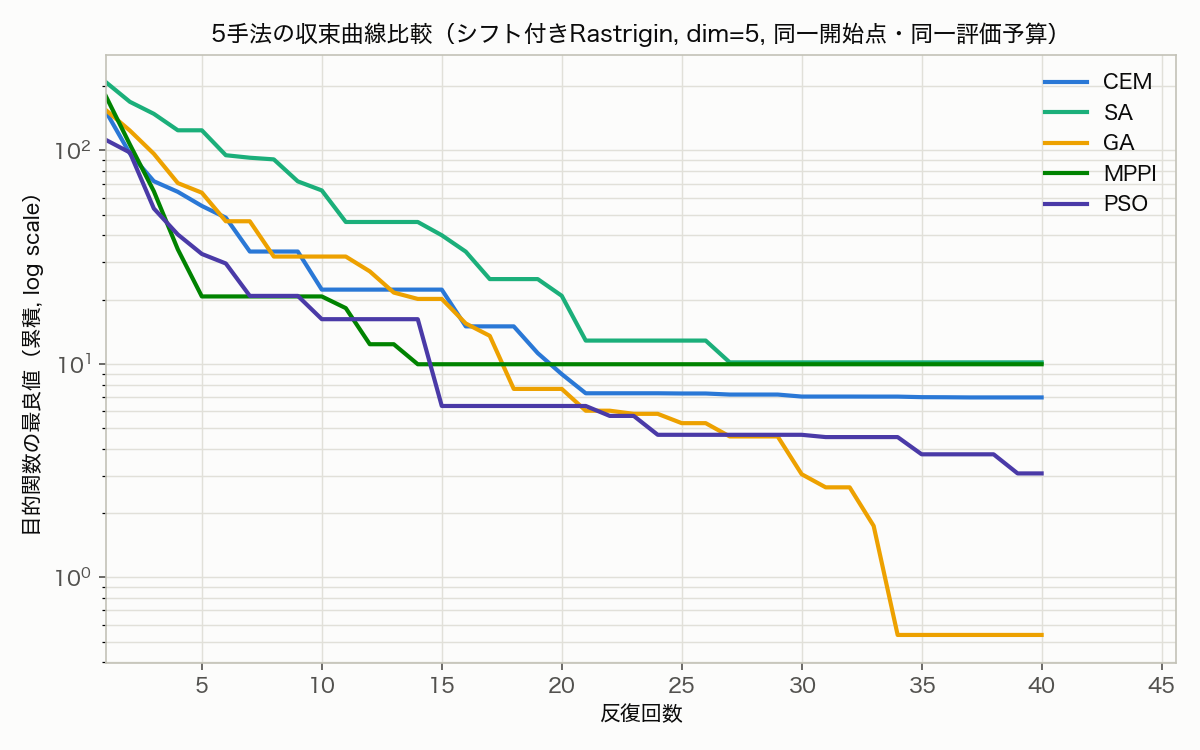
A few things stand out in the figure:
- GA reaches the lowest final value (0.537): uniform crossover preserves population diversity, producing a sharp drop around iteration 34 — likely a mutation that escaped into a different basin of the cosine’s periodic landscape
- MPPI and SA plateau early: once MPPI’s weighted average collapses onto a single basin (around iteration 15), the fixed exploration width
sigma=1.5can no longer escape it, so it flatlines at 9.96. SA behaves similarly — with a fairly aggressive cooling schedule (cooling=0.93), it stops accepting uphill moves past iteration 20 and stalls - CEM and PSO decrease steadily but end up behind GA: both refine their distribution/swarm around a single basin, making local progress without escaping the multi-modal landscape
Caveat (limits of this benchmark): this compares each method’s “default-ish” hyperparameters, not a rigorous performance benchmark. CEM’s elite_frac, SA’s cooling schedule, MPPI’s sigma, and PSO’s w, c1, c2 would all improve substantially with individual tuning (each method’s hyperparameter sensitivity is examined in its own deep-dive article, linked below). What this run actually demonstrates is the article’s core claim: the “sample → evaluate → update” loop runs all five methods without modification.
Deep-Dive Pointers per Method
CEM (Cross-Entropy Method)
Maximum-likelihood-fits the next distribution to the elite quantile, derived from KL divergence minimization. Extremely simple and widely used for RL policy search.
Read more: Cross-Entropy Method
SA (Simulated Annealing)
Anneals temperature \(T\) and probabilistically accepts uphill moves with Boltzmann probability \(\exp(-\Delta f / T)\) . A long-time standard for combinatorial problems and TSP.
Read more: Simulated Annealing
GA (Genetic Algorithms)
Evolves a population via selection, crossover, and mutation. Handles both discrete and continuous problems and is widely used in design, path planning, and feature selection.
Read more: Genetic Algorithms
MPPI (Model Predictive Path Integral)
Treats control sequences as a distribution and updates the nominal trajectory by cost-exponentially-weighted averaging. Effectively a continuous-time / continuous-control sibling of CEM, increasingly standard in real-time robotic MPC.
Read more: MPPI
PSO (Particle Swarm Optimization)
Updates particle velocities with inertia + personal-best attraction + global-best attraction. Intuitive to implement with few hyperparameters.
Read more: PSO
Bayesian Optimization
Builds a Gaussian-process surrogate and uses an acquisition function to choose the next evaluation point. Dominates the others when each evaluation is expensive.
Read more: Bayesian Optimization
Particle Filters (Sibling Method)
A state-estimation method rather than an optimizer, but its resampling mechanism is mathematically equivalent to CEM’s elite selection and MPPI’s reweighting — the original Monte Carlo family member.
Read more: Particle Filter Python Implementation
Selection Guide
Pragmatic guidance for choosing a method on a real problem:
| Situation | Recommended | Reason |
|---|---|---|
| Evaluation is very expensive (minutes+) | Bayesian optimization | Orders-of-magnitude better sample efficiency |
| Continuous opt, low–mid dim (up to tens) | CEM, PSO | Simple, fast convergence |
| Continuous opt, high dim (hundreds+) | CEM, MPPI | Parametric distribution mitigates curse of dim |
| Combinatorial opt, TSP, scheduling | SA, GA | Discrete neighborhoods / individuals are natural |
| Real-time control, robotics | MPPI | GPU-parallel sampling, 100Hz+ control loops |
| Strongly multi-modal, global optimum required | GA, multimodal CEM | Population maintains diversity |
| Some gradient information is available | Hybrid with gradient | MC for initialization → gradient method to refine |
Quick Flowchart
How expensive is f(x)?
├─ Very expensive ──> Bayesian optimization
└─ Cheap–moderate
    │
    Continuous or discrete?
    ├─ Discrete  ──> SA / GA
    └─ Continuous
        │
        Real-time required?
        ├─ Yes ──> MPPI
        └─ No
            │
            Need to exploit per-particle best history?
            ├─ Yes ──> PSO
            └─ No  ──> CEM
This is a first approximation. Hybrid strategies (e.g., coarse CEM followed by GA for diversity) are often effective in practice.
Recent Research
Treating these methods as instances of one common skeleton is itself an active research theme.
- Zhao, Q., Duan, Q., Yan, B., Cheng, S., & Shi, Y. (2023). Automated Design of Metaheuristic Algorithms: A Survey . arXiv:2303.06532 (revised February 2024). This survey treats GA, SA, PSO, and similar metaheuristics not as separate techniques but as instances drawn from a common “design space,” and organizes the methods that automatically search over hyperparameters and operator choices within that space. It backs up this article’s stance — that these algorithms differ only in the update operator \(\mathcal{U}\) — from the perspective of algorithm-design theory. The large performance gap we saw above between each method’s default settings is exactly the problem automated design/tuning tries to solve
- Poyrazoglu, O. G., Cao, Y., Moorthy, R., & Isler, V. (2026). Uncertainty Guided Exploratory Trajectory Optimization for Sampling-Based Model Predictive Control. arXiv:2604.12149. This work targets the initialization- and exploration-width sensitivity of MPPI-family sampling-based MPC, representing trajectories as distributions with uncertainty ellipsoids and enforcing sample separation via Hellinger distance (UGE-MPC) to improve sample coverage. It reports 72.1% faster convergence versus baselines in obstacle-free environments — a concrete fix for exactly the failure mode we observed above, where MPPI collapsed onto a single basin around iteration 15 and plateaued (early exploration collapse from a fixed sampling variance)
Connections to Signal Processing
Monte Carlo optimization touches signal processing in several ways:
- Non-convex adaptive filtering: when standard LMS/RLS gets stuck in local minima, CEM or GA can warm-start them
- Filter coefficient design under quantization: integer-coefficient FIR design uses SA / GA
- Control sequence optimization in MPC for signals: MPPI is increasingly standard
- State estimation: for nonlinear / non-Gaussian systems, particle filters outperform linear (Kalman) filters
In particular, MPPI naturally handles non-differentiable costs (collision avoidance, binary constraints) that classical LQR / MPC cannot, making it popular at the intersection of signal processing and control.
Summary
- All Monte Carlo optimizers share the sample → evaluate → update skeleton
- CEM / SA / GA / MPPI / PSO differ only in the update operator \(\mathcal{U}\)
- A single Python skeleton with swappable
samplerandupdaterimplements all of them - Selection by evaluation cost → continuous/discrete → real-time → history use is a practical order
- Bayesian optimization and particle filters also live in the same Monte Carlo family
See the related articles below for the full mathematics and implementations of each method.
Related Articles
- Cross-Entropy Method: A Practical Monte Carlo Optimization Technique - Importance sampling and elite-quantile distribution updates.
- Simulated Annealing: Theory and Python Implementation - Temperature scheduling and Boltzmann acceptance.
- Genetic Algorithms: Fundamentals and Python Implementation - Selection, crossover, and mutation in population evolution.
- MPPI (Model Predictive Path Integral) - Unified view with CEM and application to control.
- Particle Swarm Optimization (PSO) - Inertia weight and cognitive/social coefficients in the velocity update.
- Bayesian Optimization: Fundamentals and Python Implementation - GP surrogates and acquisition-function-based sample selection.
- Particle Filter Python Implementation - Resampling as the founding Monte Carlo mechanism.
References
- Rubinstein, R. Y., & Kroese, D. P. (2004). The Cross-Entropy Method. Springer.
- Kirkpatrick, S., Gelatt, C. D., & Vecchi, M. P. (1983). Optimization by Simulated Annealing. Science, 220(4598), 671–680.
- Holland, J. H. (1992). Adaptation in Natural and Artificial Systems. MIT Press.
- Williams, G., et al. (2017). Model Predictive Path Integral Control: From Theory to Parallel Computation. Journal of Guidance, Control, and Dynamics, 40(2).
- Kennedy, J., & Eberhart, R. (1995). Particle Swarm Optimization. Proc. IEEE ICNN.
- Shahriari, B., et al. (2016). Taking the Human Out of the Loop: A Review of Bayesian Optimization. Proc. IEEE, 104(1).
- Zhao, Q., Duan, Q., Yan, B., Cheng, S., & Shi, Y. (2023). Automated Design of Metaheuristic Algorithms: A Survey. arXiv:2303.06532.
- Poyrazoglu, O. G., Cao, Y., Moorthy, R., & Isler, V. (2026). Uncertainty Guided Exploratory Trajectory Optimization for Sampling-Based Model Predictive Control. arXiv:2604.12149.