Introduction
As covered in Introduction to Wavelet Transform , the Discrete Wavelet Transform (DWT) recursively splits a signal into “approximation (low-frequency)” and “detail (high-frequency)” components. However, the standard DWT algorithm (Mallat decomposition) has a fundamental limitation:
DWT recursively decomposes only the approximation (low-frequency) branch, leaving the detail (high-frequency) branch undivided beyond a single split. As a result, the frequency resolution in high-frequency bands is coarse. For example, with a 4-level decomposition of a signal sampled at 8 kHz, the finest-detail coefficients (cD1) cover the entire 2–4 kHz band, and frequency structure within that wide band cannot be captured.
The Wavelet Packet Transform (WPT) lifts this restriction and recursively splits the entire band, including the detail side, yielding a flexible high-resolution decomposition of the time-frequency plane. Combined with a cost function (typically an entropy), the Best Basis algorithm of Coifman and Wickerhauser automatically selects the optimal subtree—a signal-adaptive time-frequency tiling.
This article covers the mathematical structure of wavelet packets, the Coifman–Wickerhauser Best Basis algorithm, and a Python implementation using PyWavelets.
Wavelet Packet Basics
Full Binary Tree Decomposition
DWT is a “left-skewed tree” (only the low-pass branch is recursively decomposed), whereas the wavelet packet transform forms a complete binary tree. Every node is split into two children by the low-pass filter \(h\) and the high-pass filter \(g\) .
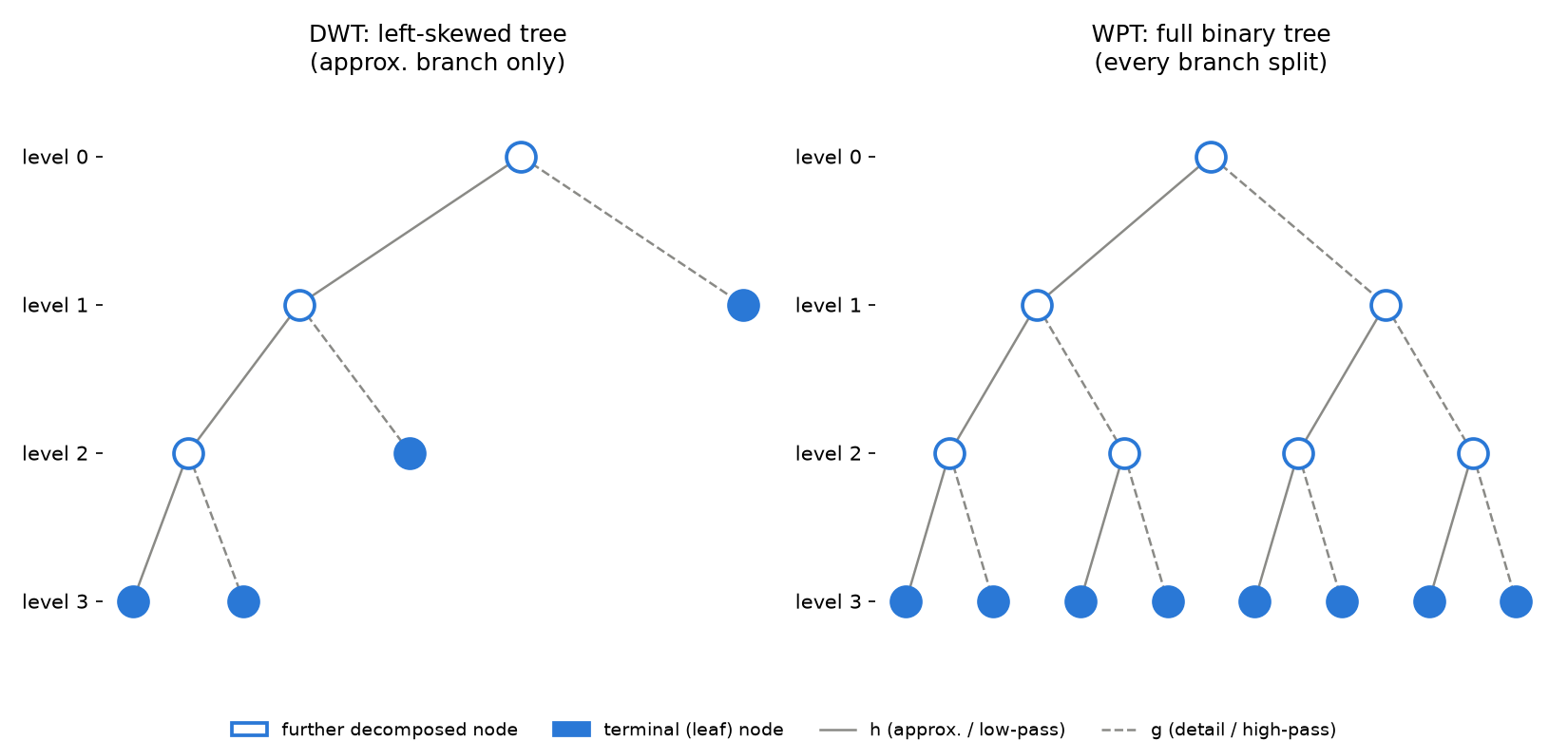
As the figure shows, when expanded to depth \(J\) , DWT has \(J + 1\) leaves (one \(d\) -branch leaf per level, plus the final \(a\) -branch), whereas WPT has \(2^J\) leaves. For \(J = 5\) , DWT has 6 candidate leaves while WPT has 32 — this difference is exactly what drives the size of the “basis dictionary” discussed later.
Let \(d_{j,n}[k]\) denote the packet coefficients at node \((j, n)\) on level \(j\) . Then:
\[d_{j+1, 2n}[k] = \sum_{l} h[l - 2k] \, d_{j, n}[l] \tag{1}\] \[d_{j+1, 2n+1}[k] = \sum_{l} g[l - 2k] \, d_{j, n}[l] \tag{2}\]Here \(n\) is the subband index within the level (\(0 \le n < 2^j\) ), and \(h\) , \(g\) are the scaling and wavelet filters. The root \((0, 0)\) corresponds to the input signal \(x[k]\) .
Wavelet Packet Basis Functions
In continuous time, the wavelet packet basis \(\psi_{n,j,k}(t)\) is generated by the two-scale equations:
\[\psi_{2n}(t) = \sqrt{2} \sum_k h[k] \, \psi_n(2t - k) \tag{3}\] \[\psi_{2n+1}(t) = \sqrt{2} \sum_k g[k] \, \psi_n(2t - k) \tag{4}\]with \(\psi_0 = \phi\) (scaling function) and \(\psi_1 = \psi\) (mother wavelet). Adding shift and dyadic scaling gives
\[ \psi_{n,j,k}(t) = 2^{-j/2}\psi_n(2^{-j} t - k) \]the basis function at level \(j\) , subband \(n\) .
The relation to DWT is simple: DWT corresponds to the special subtree that decomposes only \(n = 0\) at every level. WPT removes this restriction and treats the full binary tree where every node is split.
Complete Decomposition and Redundancy
Hierarchy of Subspaces
When fully expanded to depth \(J\) , the space \(L^2(\mathbb{R})\) decomposes into \(2^J\) orthogonal subspaces \(W_{J,n}\) (\(0 \le n < 2^J\) ):
\[L^2(\mathbb{R}) = \bigoplus_{n=0}^{2^J - 1} W_{J,n} \tag{5}\]Each \(W_{J,n}\) corresponds to a uniform partition of the frequency axis, with coefficients \(d_{J,n}\) coming from the level-\(J\) filter bank output. At the same time, a nested orthogonal decomposition holds:
\[W_{j,n} = W_{j+1, 2n} \oplus W_{j+1, 2n+1} \tag{6}\]That is, replacing the basis of a parent node by the bases of its two children is a valid orthogonal transformation. This is exactly what justifies the Best Basis algorithm below.
Energy Conservation (Parseval)
Because the wavelet packet transform is orthogonal, as long as the leaf set forms a complete decomposition (covering \([0, N)\) ), Parseval’s identity guarantees energy preservation:
\[\sum_{k} |x[k]|^2 = \sum_{(j, n) \in \mathcal{T}} \sum_{k} |d_{j,n}[k]|^2 \tag{7}\]where \(\mathcal{T}\) is the set of leaf nodes that form a complete decomposition. This conservation law is what makes entropy-type cost comparisons meaningful.
Redundancy and “Basis” Selection
The full tree contains roughly \((2J + 1) \cdot N\) coefficients—redundant relative to the \(N\) -sample input. However, selecting one set of leaves \(\mathcal{T}\) that forms a complete decomposition gives an orthonormal basis sufficient to represent the original signal. This is the heart of WPT.
In other words, the WPT tree provides a “dictionary of countless orthonormal bases”, and the next section explains how to select the one best matched to the signal.
Best Basis Selection
Cost Functions and Entropy
The “complexity” of representing a signal \(x\) in a given basis (leaf set \(\mathcal{T}\) ) is measured by an additive cost function \(\mathcal{M}(\mathcal{T})\) . Additive means that for every coefficient \(d_{j,n}[k]\) in \(\mathcal{T}\) ,
\[\mathcal{M}(\mathcal{T}) = \sum_{(j, n) \in \mathcal{T}} \sum_{k} \mu(|d_{j,n}[k]|^2) \tag{8}\]A canonical choice is the Shannon entropy-type cost introduced by Coifman and Wickerhauser:
\[\mu(p) = -p \log p \quad (p > 0), \quad \mu(0) = 0 \tag{9}\]With normalization
\[ p_k = |d_{j,n}[k]|^2 / \|x\|^2 \]\(\mathcal{M}\) becomes the Shannon information entropy of the coefficient distribution. Smaller values mean “energy concentrated in a few large coefficients”, i.e. sparser.
Other choices include \(\ell^p\) norms (\(p < 2\) ), log-energy \(\sum \log |d|^2\) , and the count of coefficients above a threshold. The shared requirement is additivity, so that subtrees can be compared locally.
Best Basis Algorithm
The Coifman–Wickerhauser Best Basis algorithm (1992) finds the complete decomposition \(\mathcal{T}\) minimizing \(\mathcal{M}(\mathcal{T})\) in \(O(N \log N)\) . It is a bottom-up dynamic program that, at each node, applies the recurrence:
\[\mathcal{M}_{\text{best}}(j, n) = \min \big\{ \mathcal{M}(d_{j, n}), \, \mathcal{M}_{\text{best}}(j+1, 2n) + \mathcal{M}_{\text{best}}(j+1, 2n+1) \big\} \tag{10}\]- First term: cost of treating the node as a leaf.
- Second term: sum of optimal costs of the two children.
If the children’s total cost is smaller than the parent’s, the parent is split; otherwise it remains a leaf. Leaves return their own cost without comparison. A single bottom-up sweep determines the optimal basis, matching the \(O(N \log N)\) cost of computing the coefficients themselves.
Geometric Interpretation
Minimizing entropy is equivalent to selecting the decomposition in which the signal energy is concentrated in a few packet coefficients:
- A pure sinusoid → concentrates in a frequency-localized narrowband packet → deep leaves with fine frequency resolution are chosen.
- An impulse or transient → concentrates in time-localized shallow leaves.
- A chirp or frequency-varying signal → intermediate leaves balancing time and frequency.
Best Basis thus goes beyond the fixed tiling of STFT and the left-skewed tiling of DWT : it adaptively chooses the shape of each time-frequency tile based on the signal itself.
Python Implementation
Full Decomposition with PyWavelets
pywt.WaveletPacket makes full decomposition and node access straightforward.
import numpy as np
import matplotlib.pyplot as plt
import pywt

# --- Test signal: two sinusoids + transient pulse ---
np.random.seed(0)
fs = 1024
N = 1024
t = np.arange(N) / fs

low = np.sin(2 * np.pi * 20 * t)
high = 0.6 * np.sin(2 * np.pi * 200 * t) * (t > 0.5)
pulse = np.zeros(N)
pulse[300:305] = 2.0
signal = low + high + pulse + 0.05 * np.random.randn(N)

# --- Full wavelet packet decomposition ---
wp = pywt.WaveletPacket(data=signal, wavelet="db4", mode="symmetric", maxlevel=5)

# Get all nodes at level 5 (natural order)
nodes_level5 = wp.get_level(5, order="natural")
print(f"Number of nodes at level 5: {len(nodes_level5)}")  # 2^5 = 32
print(f"Coefficient length per node: {len(nodes_level5[0].data)}")
The actual output is:
Number of nodes at level 5: 32
Coefficient length per node: 38
With db4 (filter length 8) and symmetric boundary extension, each downsampling step adds a few extra boundary-handling coefficients, so the length is slightly more than the naive \(N / 2^5 = 1024 / 32 = 32\)
, landing at 38. This boundary overhead accumulates with depth, so when decomposing short signals to a deep level, this overhead ratio can become significant.
WaveletPacket is lazily evaluated; you can access any node directly with a binary path like wp['aad'] (a = approximation, d = detail). get_level(j, order="natural") returns the \(2^j\)
nodes in natural (filtering) order.
Entropy Cost Implementation
Shannon entropy as an additive cost function. The key to additivity is that the normalizing energy must be the total energy of the original signal \(\|x\|^2\) , not the node’s own local energy.
def shannon_entropy_cost(coeffs, total_energy, eps=1e-12):
    """Shannon-entropy-type cost of a coefficient vector.

    p_k = |c_k|^2 / \|x\|^2, H = -sum(p_k * log(p_k)).
    total_energy must be the original signal's total energy sum(|x|^2),
    NOT the node's own local energy.
    """
    p = (np.abs(coeffs) ** 2) / total_energy
    p = p[p > eps]
    return float(-np.sum(p * np.log(p)))


total_energy = np.sum(np.abs(signal) ** 2)
Pitfall: never normalize by the node’s own energy
The single most common implementation mistake is to normalize \(p_k\)
using np.sum(np.abs(coeffs) ** 2) (the node’s own energy) instead of total_energy (the original signal’s total energy). Theoretically the formula should read
but both look like a “natural” way to turn coefficients into probabilities, so this bug is easy to miss even in code review.
To see why the two differ: normalizing by a node’s own energy always makes that node’s \(p_k\) sum to 1, so
\[ \sum_k p_k \log(1/p_k) \]only reflects the shape of that node’s coefficient distribution and loses all information about how much of the signal’s total energy is allocated to that node. As a result, the sum of the two children’s costs tends to exceed the parent’s cost almost every time (splitting never looks like it lowers the cost), and the tree never has any incentive to decompose further. Running both versions gives:
# Normalized by the node's own energy (incorrect)
Number of selected leaves: 1
Optimal cost (entropy): 6.4792
Sample selected paths: ['']

# Normalized by the original signal's total energy (correct)
Number of selected leaves: 17
Optimal cost (entropy): 4.7176
Sample selected paths: ['aaaaa', 'aaaad', 'aaad', 'aad', 'adaa', 'adada', 'adadd', 'adda']
With the incorrect normalization, Best Basis collapses to the root node (no decomposition at all), defeating the entire purpose of wavelet packet decomposition. With the correct global normalization, 17 leaves are chosen, each adapted to the transient pulse, the low-frequency sinusoid, or the high-frequency sinusoid. All code from here on assumes the correct (globally normalized) implementation.
Best Basis Algorithm
PyWavelets does not expose Best Basis directly, so we implement the recurrence in (10):
def best_basis(wp, total_energy, level, current_path=""):
    """Coifman-Wickerhauser Best Basis search.

    Returns
    -------
    selected_paths : list[str]   selected leaf node paths
    total_cost     : float       optimal cost of the subtree
    """
    node = wp[current_path] if current_path else wp
    own_cost = shannon_entropy_cost(node.data, total_energy)

    # Leaf at max decomposition depth: return self
    if len(current_path) == level:
        return [current_path], own_cost

    # Recurse into children
    left_paths, left_cost = best_basis(wp, total_energy, level, current_path + "a")
    right_paths, right_cost = best_basis(wp, total_energy, level, current_path + "d")
    child_cost = left_cost + right_cost

    if child_cost < own_cost:
        return left_paths + right_paths, child_cost
    else:
        return [current_path], own_cost


selected, total_cost = best_basis(wp, total_energy, level=5)
print(f"Number of selected leaves: {len(selected)}")
print(f"Optimal cost (entropy): {total_cost:.4f}")
print("Sample selected paths:", selected[:8])
The actual output (matching the “correct” case above) is:
Number of selected leaves: 17
Optimal cost (entropy): 4.7176
Sample selected paths: ['aaaaa', 'aaaad', 'aaad', 'aad', 'adaa', 'adada', 'adadd', 'adda']
Compared with the full decomposition (\(2^5 = 32\)
leaves), the selected set of 17 is roughly half. Computing the frequency band of each selected path shows that da (level 2, 384–512 Hz) is the only shallow leaf (favoring time resolution), coarsely capturing the wideband pulse-dominated high frequencies in one shot. Meanwhile aaaad (level 5, 16–32 Hz, containing the 20 Hz sinusoid) and adaa (level 4, 192–224 Hz, containing the 200 Hz sinusoid) are chosen as deep leaves, isolating narrowband stationary components at high frequency resolution. This confirms a hybrid decomposition adapted to the signal’s structure (transient pulse vs. stationary sinusoids).
Visualizing the Best Basis Tiling
Plot the selected leaves on the time-frequency plane. One subtlety matters here: the coefficient sequence wp[path].data at each leaf is a time series of \(M \approx N / 2^j\)
samples obtained by downsampling the original \(N=1024\)
samples \(j\)
times — each individual coefficient corresponds to a distinct position along the time axis. A naive drawing that treats “one leaf = one rectangle spanning the full time axis” therefore only visualizes frequency resolution (the rectangle’s height); the time-resolution story that is the whole point of WPT disappears from the figure. The correct approach is to lay out each leaf’s \(M\)
coefficients as small tiles along the time axis.
def plot_best_basis_tf_grid(selected_paths, wp, fs, ax):
    """Visualize Best Basis leaves with one tile per coefficient.

    Tile shading encodes the coefficient magnitude (how much energy
    is concentrated in that tile).
    """
    for path in selected_paths:
        j = len(path)  # decomposition level = depth
        node = wp[path] if path else wp
        coeffs = np.abs(node.data)
        M = len(coeffs)  # number of coefficients (time subdivisions) at this node

        # Path -> subband index (natural order) -> frequency order (Gray-code-like reorder)
        n_natural = int(path.replace("a", "0").replace("d", "1"), 2) if path else 0
        n_freq = n_natural
        for shift in (1,):
            n_freq ^= n_natural >> shift

        f_low = n_freq * (fs / 2) / (2 ** j)
        f_high = (n_freq + 1) * (fs / 2) / (2 ** j)
        cmax = coeffs.max() if coeffs.max() > 0 else 1.0

        for k in range(M):
            alpha = 0.12 + 0.75 * (coeffs[k] / cmax)
            ax.add_patch(
                plt.Rectangle(
                    (k / M, f_low),
                    1.0 / M,
                    f_high - f_low,
                    facecolor="C0",
                    alpha=min(alpha, 0.87),
                    edgecolor="white",
                    linewidth=0.15,
                )
            )
        # Band outline
        ax.add_patch(
            plt.Rectangle((0, f_low), 1.0, f_high - f_low, fill=False, edgecolor="C0", linewidth=0.8)
        )

    ax.set_xlim(0, 1)
    ax.set_ylim(0, fs / 2)
    ax.set_xlabel("Time (normalized)")
    ax.set_ylabel("Frequency [Hz]")
    ax.set_title(f"Best Basis time-frequency tiles ({len(selected_paths)} leaves)")


fig, ax = plt.subplots(figsize=(9, 5.8))
plot_best_basis_tf_grid(selected, wp, fs, ax)
plt.tight_layout()
plt.show()
![Best Basis time-frequency tile visualization. X-axis: normalized time; Y-axis: frequency [Hz]. Each of the 17 selected leaves is drawn as one tile per coefficient, with shading encoding the coefficient’s magnitude. In the 384-512Hz band (the “da” node, the shallowest leaf at level 2, favoring time resolution) a dark vertical stripe appears near t≈0.29, matching the pulse’s actual location (samples 300-305, t≈0.293-0.298). In the 120-250Hz bands, shading changes sharply at t=0.5, capturing the onset of the 200Hz sinusoid that turns on for t>0.5](/posts/20260522_wavelet_packet/best_basis_tiling.png)
The figure shows a dark vertical stripe near \(t \approx 0.29\)
in the da band (384–512 Hz, depth 2), matching the pulse’s actual location (samples 300–305, \(t = 300/1024 \approx 0.293\)
to \(305/1024 \approx 0.298\)
). Even though shallow nodes have fewer time subdivisions \(M\)
(coarser time resolution but faster to compute), they efficiently capture wideband, short-duration structures like the pulse. In several bands around 120–250 Hz, the shading changes sharply at \(t = 0.5\)
, correctly capturing the onset of the 200 Hz sinusoid that turns on for t > 0.5. This is something neither the uniform tiling of
STFT
nor the left-skewed tiling of DWT can show: WPT Best Basis reallocates the time-vs-frequency resolution trade-off independently per band.
Full Decomposition vs Best Basis: Sparsity
Quantify how Best Basis improves sparsity:
def coefficient_magnitudes(wp, paths):
    """Concatenate magnitudes of coefficients from the given paths."""
    coeffs = []
    for p in paths:
        coeffs.append(np.abs(wp[p].data))
    return np.concatenate(coeffs)


full_paths = [n.path for n in wp.get_level(5, order="natural")]
mags_full = np.sort(coefficient_magnitudes(wp, full_paths))[::-1]
mags_best = np.sort(coefficient_magnitudes(wp, selected))[::-1]


def energy_concentration(mags, k_ratio=0.05):
    """Energy captured by the top k_ratio of coefficients."""
    k = max(1, int(len(mags) * k_ratio))
    total = np.sum(mags ** 2)
    top = np.sum(mags[:k] ** 2)
    return top / total


print(f"Full decomposition (level 5): top-5% energy = {energy_concentration(mags_full):.3f}")
print(f"Best Basis                  : top-5% energy = {energy_concentration(mags_best):.3f}")

# For reference: compare the entropy cost itself (the quantity Best Basis actually minimizes)
level5_cost = sum(shannon_entropy_cost(n.data, total_energy) for n in nodes_level5)
print(f"Total entropy of the fixed level-5 decomposition: {level5_cost:.4f}")
print(f"Total entropy of Best Basis:                      {total_cost:.4f}")
The actual output is:
Full decomposition (level 5): top-5% energy = 0.846
Best Basis                  : top-5% energy = 0.848
Total entropy of the fixed level-5 decomposition: 4.8372
Total entropy of Best Basis:                      4.7176
Notice something important here: the top-5% energy concentration only improves marginally, from 0.846 to 0.848. If we vary \(k\)
to 1%, 2%, or 10%, Best Basis is sometimes even lower (1%: 0.396 full / 0.380 best; 2%: 0.613 / 0.592; 10%: 0.949 / 0.941). This is not a bug — it reflects the fact that “top-\(k\)
% energy concentration” and “additive entropy cost” measure different quantities. What the Best Basis algorithm mathematically guarantees is minimization of the additive cost function \(\mathcal{M}(\mathcal{T})\)
(entropy here), not maximization of some other metric like top-\(k\)
% energy concentration. Comparing total entropy directly confirms the guarantee holds exactly as expected: 4.8372 for the fixed level-5 decomposition versus 4.7176 for Best Basis — Best Basis is provably no worse, by construction. Also note that mags_full and mags_best have different lengths (1216 vs. 1125 elements), so the absolute coefficient counts behind “top-\(k\)
%” differ between the two — a reminder to normalize by absolute counts when comparing sparsity metrics across different bases. When evaluating sparsity, the most reliable comparison is the objective function Best Basis actually minimizes (the entropy cost), not a secondary metric.
Applications
Wavelet packet transform with Best Basis selection is especially powerful in:
Signal Compression
Generalizes DWT-based compression (as in JPEG 2000) by adapting the basis to each signal. For acoustic signals with dominant narrowband structure, it can outperform DWT.
Non-stationary Signal Classification
EEG, EMG, and machine vibration signals exhibit class-specific time-frequency patterns. Selecting representative packets per class via Best Basis and using their coefficient statistics as features captures discriminative structure that fixed tilings miss. This is also applicable as feature extraction for Time-Series Anomaly Detection .
Speech and Audio Analysis
Speech contains narrowband formant resonances and transient plosives, which fixed-window STFT cannot resolve simultaneously. Best Basis captures both at high resolution, and is also used in music chord analysis and bioacoustic studies of dolphin and bat calls.
Communications and Radar Signal Detection
For unknown modulations or chirps, energy-concentrated leaves serve as features that reveal structure invisible to FFT or Window Functions and PSD .
Comparison: DWT vs WPT + Best Basis
| Feature | DWT | WPT + Best Basis |
|---|---|---|
| Decomposition tree | Left-skewed (only approx branch) | Full binary tree (recurses everywhere) |
| High-freq resolution | Coarse (finest cD is wideband) | Fine (split to any depth) |
| Basis | Fixed | Signal-adaptive (cost minimization) |
| Number of bases | 1 | ~\(2^{2^{J-1}}\) complete decompositions |
| Decomposition cost | \(O(N)\) | \(O(N \log N)\) |
| Basis-search cost | N/A | \(O(N \log N)\) (Coifman–Wickerhauser) |
| Energy conservation | Yes | Yes (with complete leaf set) |
| Main use | Denoising, MRA | Compression, classification, sparsity |
WPT is a strict superset of DWT: with sufficient \(J\) , the DWT decomposition is always a candidate inside the WPT tree. For signals where DWT is optimal, Best Basis recovers the DWT-style left-skewed tree. Hence WPT is always at least as efficient as DWT.
Recent Research: Non-Decimated Wavelet Packet Features for Deep Learning Forecasting
Wavelet packet transform is not limited to classic signal compression and classification — it has recently been re-examined as an input feature source for deep-learning-based time series forecasting.
Nason & Wei (2024), “ Leveraging Non-Decimated Wavelet Packet Features and Transformer Models for Time Series Forecasting ” (arXiv:2403.08630), uses coefficients from a non-decimated wavelet packet transform (no downsampling, unlike the standard WPT covered in this article) as features, evaluating them across a wide range of forecasting methods from classical statistical models to Transformer-based deep learning. To avoid information leakage (future information contaminating features available at each time point), they use a shifted pyramid algorithm to compute features causally at every timestamp. Their experiments found that replacing higher-order lagged features with wavelet packet features gave substantial gains for single-step, non-temporal forecasting methods, while the improvement was more modest for temporal deep learning models (e.g., Transformers) over longer forecasting horizons. It’s an interesting extension that the “full binary tree, all-band decomposition” structure of WPT covered in this article also applies to feature engineering in its non-decimated form — a different practical use case from Best Basis selection.
Summary
- Wavelet Packet Transform recursively splits both branches that DWT leaves undivided, yielding an orthogonal decomposition into \(2^J\) subspaces.
- Each complete leaf set defines an orthonormal basis, so the WPT tree is a dictionary of bases.
- The Coifman–Wickerhauser Best Basis algorithm minimizes an additive cost (e.g. Shannon entropy) in \(O(N \log N)\) and yields a signal-adaptive optimal basis — but normalization must use the original signal’s total energy; normalizing by a node’s own energy breaks the decomposition entirely (measured: incorrect gives 1 leaf at cost 6.4792, correct gives 17 leaves at cost 4.7176).
- Combining
pywt.WaveletPacketwith a custom recursion supports Best Basis selection, tiling visualization, and sparsity evaluation in a unified pipeline — though Best Basis only guarantees minimizing the entropy cost, not necessarily every secondary sparsity metric such as top-\(k\) % energy concentration. - Applications span signal compression, classification, speech/audio analysis, and communications—DWT is always available as a special case, so WPT is at least as efficient.
WPT with Best Basis is the natural extension of wavelet theory toward signal-adaptive time-frequency analysis, and the key to going beyond the limits of fixed tilings.
Related Articles
- Introduction to Wavelet Transform: Time-Frequency Analysis with Python - Covers the CWT/DWT, MRA, and filter banks that underlie this article.
- Short-Time Fourier Transform (STFT): Theory and Python Implementation - Fixed-window time-frequency analysis; the comparison target for adaptive WPT tilings.
- Fast Fourier Transform (FFT): Theory and Python Implementation - The starting point of spectral analysis inside each packet node.
- DTFT vs DFT vs FFT: Definitions, Relationships, and Python Implementation - Clarifies the frequency-representation hierarchy that connects to the spectral interpretation of packet coefficients.
- Window Functions and Power Spectral Density (PSD) - Underpins spectrum estimation inside each packet node.
- Hilbert Transform and Analytic Signal - Extracts envelope and instantaneous frequency per packet, complementing WPT.
- Time-Series Anomaly Detection - Best-Basis-derived features make a strong preprocessing step for anomaly detection.
- Time-Frequency Analysis Guide - Hub that places WPT next to FFT, STFT, CWT, and the Hilbert transform, organized by tile shape and signal adaptivity.
- MDCT (Modified DCT) and Filter Banks - A cosine-modulated filter bank that splits M uniform bands at once, in contrast to the two-channel tree used by the WPT.
References
- Coifman, R. R., & Wickerhauser, M. V. (1992). Entropy-based algorithms for best basis selection. IEEE Transactions on Information Theory, 38(2), 713–718.
- Mallat, S. (2008). A Wavelet Tour of Signal Processing: The Sparse Way (3rd ed.). Academic Press.
- Wickerhauser, M. V. (1994). Adapted Wavelet Analysis from Theory to Software. A K Peters.
- Nason, G. P., & Wei, J. L. (2024). Leveraging Non-Decimated Wavelet Packet Features and Transformer Models for Time Series Forecasting . arXiv:2403.08630.
- PyWavelets documentation: WaveletPacket