Introduction
Time-frequency analysis is the umbrella name for techniques that estimate which frequencies are present in a signal, when they occur, and how strong they are at each instant. The flagship methods are the FFT , the STFT , the continuous and discrete wavelet transforms (CWT/DWT) , the wavelet packet transform , the Hilbert transform , and the Hilbert-Huang transform (EMD followed by Hilbert spectral analysis). Each method has different assumptions, resolution trade-offs, computational cost, and signal classes for which it shines.
This article is a hub designed to answer the question: given my signal and goal, which method should I reach for, and with what parameters? We organize the landscape along three selection axes, summarize the methods in a feature matrix, walk through nine common application scenarios, and provide a unified Python evaluation framework that runs five methods side-by-side on the same chirp. Detailed derivations live in the per-method articles linked from this hub; this article keeps the map. Read it next to the Bode plot hub —its twin from the LTI-system design side—and you have a complete view of the frequency domain.
Three Selection Axes
Axis 1: Time resolution vs. frequency resolution (Heisenberg trade-off)
Any analysis window obeys the uncertainty principle
\[\Delta t \cdot \Delta f \ge \frac{1}{4\pi} \tag{1}\]so a short time window blurs frequency content, and a fine frequency grid blurs time. Each method sits at a different point on this curve.
- FFT sacrifices all time information for the sharpest possible frequency resolution. Intended for stationary signals.
- STFT uses a fixed window, giving uniform time-frequency resolution across the entire band.
- CWT scales the window with frequency: short at high frequencies, long at low frequencies. This is multi-resolution analysis.
- Hilbert transform estimates the instantaneous amplitude and frequency at every sample. The time resolution is effectively one sample, but the signal must be narrowband.
Axis 2: Linear (FFT / STFT / Wavelet) vs. nonlinear (Hilbert-Huang)
A linear transform \(\mathcal{T}\) satisfies the superposition principle, \(\mathcal{T}(ax + by) = a\mathcal{T}(x) + b\mathcal{T}(y)\) . The FFT, STFT, CWT, DWT, and the wavelet packet transform are all linear—they project the signal onto fixed basis functions chosen a priori.
The Hilbert-Huang transform (HHT) is fundamentally different. Its first stage, EMD (Empirical Mode Decomposition), extracts a small set of Intrinsic Mode Functions (IMFs) directly from the data, in a way that depends on the signal itself. This makes HHT applicable to nonlinear and non-stationary signals where no fixed basis works well, at the cost of rigorous mathematical foundations.
Axis 3: Stationary vs. non-stationary signals
- Stationary: statistics (mean, variance, spectrum) do not change over time → FFT with windowing and PSD is enough.
- Quasi-stationary: stationary on short segments (speech is stationary on 20–30 ms windows) → STFT .
- Non-stationary: frequency content changes over time (chirps, transients) → CWT , wavelet packet , or HHT.
Smoothing and detrending tools such as the moving average and the exponential moving average (EMA) act as low-pass filters along the time axis and serve as common pre-processing before any of the above transforms.
Deriving the Uncertainty Bound (the Gabor Limit)
The bound \(1/(4\pi)\) in Eq. (1) is quoted, not proven, in the STFT article and the wavelet article . As the hub that ties every method back to this one constant, we derive it here.
Let \(x(t)\) be an energy-normalized signal, \(\int |x(t)|^2 dt = 1\) , with Fourier transform \(X(f)\) ; Parseval’s theorem gives \(\int |X(f)|^2 df = 1\) . Define the time and frequency spreads as variances (the centroids can always be set to zero by a time shift and a modulation, so this costs no generality):
\( \Delta t^2 = \int t^2 |x(t)|^2 \, dt, \qquad \Delta f^2 = \int f^2 |X(f)|^2 \, df \)
Integrate the normalization condition \(\int |x(t)|^2 dt = 1\) by parts:
\( 1 = \Big[t |x(t)|^2\Big]_{-\infty}^{\infty} - \int t \frac{d}{dt}|x(t)|^2 \, dt \)
Assuming \(x(t) \to 0\) fast enough that the boundary term vanishes:
\( 1 = -\int t \left( x(t)\overline{x'(t)} + \overline{x(t)} x'(t) \right) dt = -2\int t\, \mathrm{Re}\!\left[\overline{x(t)}\, x'(t)\right] dt \)
Apply the Cauchy-Schwarz inequality to \(t\,x(t)\) and \(x'(t)\) :
\( \left| \int t\, \overline{x(t)}\, x'(t)\, dt \right| \le \left( \int t^2 |x(t)|^2 dt \right)^{1/2} \left( \int |x'(t)|^2 dt \right)^{1/2} = \Delta t \cdot \left( \int |x'(t)|^2 dt \right)^{1/2} \)
The differentiation rule for the Fourier transform, \(\mathcal{F}[x'(t)] = i2\pi f\, X(f)\) , combined with Parseval’s theorem, gives
\( \int |x'(t)|^2 dt = \int (2\pi f)^2 |X(f)|^2 \, df = 4\pi^2 \Delta f^2 \)
Combining the three results:
\( 1 \le 2\left|\int t\,\overline{x(t)}\, x'(t)\, dt\right| \le 2\, \Delta t \cdot 2\pi \Delta f = 4\pi\, \Delta t\, \Delta f \)
which gives \(\Delta t \cdot \Delta f \ge 1/(4\pi)\) — Eq. (1). Equality holds exactly when the Cauchy-Schwarz step is tight, i.e. \(x'(t) \propto t\,x(t)\) ; solving this ODE yields the Gaussian \(x(t) = e^{-at^2}\) (\(a > 0\) ) as the unique minimizer. This is why the Morlet wavelet — a Gaussian-modulated complex sinusoid — is called jointly optimal in time and frequency: it sits exactly on the bound this derivation just proved. Rectangular windows and other fixed STFT windows leave slack against this bound (\(\sigma_t \sigma_f\) strictly greater than \(1/(4\pi)\) ).
Feature Comparison Matrix
| Method | Time localization | Frequency localization | Complexity | Signal class | Typical uses |
|---|---|---|---|---|---|
| FFT | none | maximal (\(1/N\) ) | \(O(N \log N)\) | stationary | spectrum, PSD, harmonic analysis |
| STFT | medium (window) | medium (\(1/L\) ) | \(O(N \log L)\) | quasi-stationary | speech, spectrograms |
| CWT | high at high freq. | high at low freq. | \(O(N \log N)\) | non-stationary | transients, singularities, biosignals |
| DWT | octave-graded | octave-graded | \(O(N)\) | non-stationary | compression, denoising |
| Wavelet packet | medium–high (adaptive) | medium–high (adaptive) | \(O(N \log N)\) | non-stationary | best-basis selection, feature extraction |
| Hilbert transform | maximal (per sample) | single (narrowband) | \(O(N \log N)\) | narrowband AM/FM | instantaneous amplitude/frequency, demod |
| Hilbert-Huang (EMD + HSA) | maximal | adaptive (per IMF) | \(O(N \cdot M)\) | nonlinear / non-stationary | biosignals, seismology, oceanography |
Here \(L\) is the STFT window length and \(M\) is the number of EMD sifting iterations.
Decision Flow: Nine Scenarios
- Pure spectrum estimation (e.g., identifying harmonics of motor excitation) → FFT with a Hann/Blackman window and Welch’s method .
- Transient analysis (impact response, defect detection) → CWT with a Morlet mother wavelet, or wavelet packet .
- Narrowband tone extraction and demodulation (AM/FM, PLL front-ends) → Hilbert transform after a tight bandpass filter.
- Mode decomposition (separating coexisting vibration modes) → EMD followed by Hilbert spectral analysis (HHT).
- Speech and speaker analysis (formants, F0 tracking) → STFT with the canonical 25 ms window and 10 ms hop.
- Mechanical vibration diagnostics (bearing faults, gear mesh) → envelope analysis with the Hilbert transform followed by FFT of the envelope.
- Biosignals (ECG, EEG, EMG) → CWT or HHT, both of which handle non-stationarity and nonlinearity well.
- Image and other 2D signals (feature extraction, compression) → 2D DWT .
- Detrending and pre-processing (high-frequency noise suppression) → moving average or EMA before any of the above.
A practical heuristic: try FFT first; if you need time localization, switch to STFT; if STFT is too rigid, switch to wavelets; if you need instantaneous quantities, switch to Hilbert. This order matches the cost of complexity and rarely overshoots.
Unified Evaluation Framework: Five Methods on One Chirp
A linear chirp—where the instantaneous frequency rises linearly with time—plus a stationary tone is a standard stress test for time-frequency methods. Rather than eyeballing plots, we have each method track the chirp’s true instantaneous frequency \(f(t) = 10 + 190t/T\) Hz and measure the actual error.
import numpy as np
from scipy.signal import chirp, spectrogram, hilbert, butter, filtfilt
import pywt

np.random.seed(0)
fs = 1000  # sampling rate [Hz]
T = 2.0    # duration [s]
t = np.linspace(0, T, int(fs * T), endpoint=False)

# 10 Hz -> 200 Hz linear chirp plus a steady 100 Hz tone, with noise
x = chirp(t, f0=10, f1=200, t1=T, method="linear") + 0.5 * np.sin(2 * np.pi * 100 * t)
x += 0.1 * np.random.randn(len(t))

true_if = 10 + (200 - 10) * t / T  # ground-truth instantaneous frequency of the chirp
(1) FFT: the spectrum is visible, but “when” is gone
X = np.fft.rfft(x)
f = np.fft.rfftfreq(len(x), 1 / fs)
mag_db = 20 * np.log10(np.abs(X) + 1e-12)
band_mask = (f >= 90) & (f <= 110)
print(f"peak near 100 Hz: {f[band_mask][np.argmax(mag_db[band_mask])]:.2f} Hz @ {mag_db[band_mask].max():.1f} dB")
print(f"noise floor (median, f>300 Hz): {np.median(mag_db[f > 300]):.1f} dB")
Output:
peak near 100 Hz: 100.00 Hz @ 54.0 dB
noise floor (median, f>300 Hz): 11.9 dB
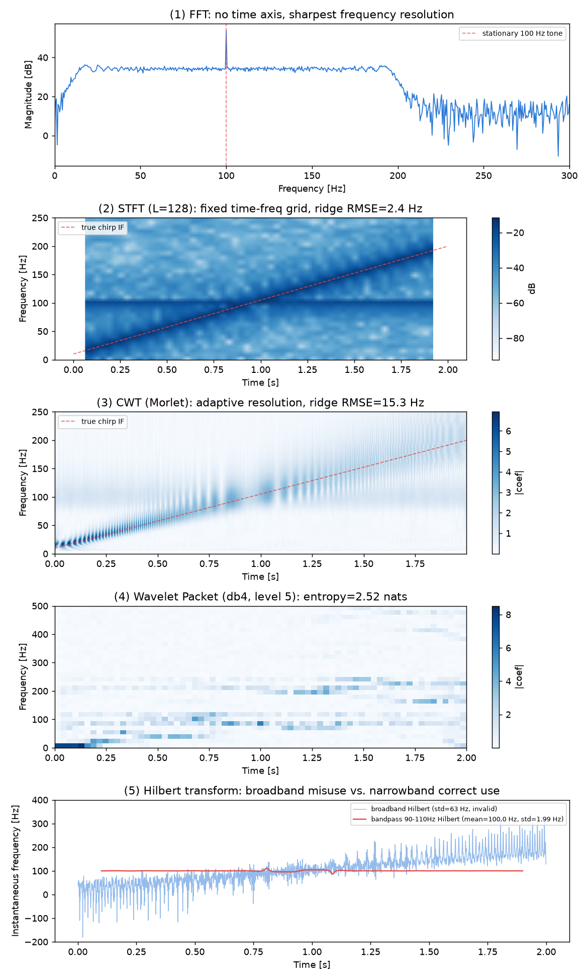
The FFT locks onto the stationary 100 Hz tone as a sharp 54.0 dB peak, but the 10→200 Hz chirp produces no peak at all — just a roughly 34 dB plateau spread across the whole 10–200 Hz band (panel (1) below). Whatever time-localized structure existed in the chirp is gone by construction.
(2)(3) STFT vs. CWT: measuring the resolution trade-off with ridge-tracking error
# STFT: fixed-window ridge (the frequency of maximum power at each time frame)
f_s, t_s, Sxx = spectrogram(x, fs, nperseg=128, noverlap=96)
ridge_f_stft = f_s[np.argmax(Sxx, axis=0)]
true_if_stft = np.interp(t_s, t, true_if)
rmse_stft = np.sqrt(np.mean((ridge_f_stft - true_if_stft) ** 2))

# CWT: ridge with log-spaced scales (5-300 Hz)
freq_lo, freq_hi = 5, 300
s_lo = pywt.frequency2scale("morl", freq_hi / fs)
s_hi = pywt.frequency2scale("morl", freq_lo / fs)
scales = np.geomspace(s_lo, s_hi, 128)
coef, freqs_cwt = pywt.cwt(x, scales, "morl", sampling_period=1 / fs)
ridge_f_cwt = freqs_cwt[np.argmax(np.abs(coef), axis=0)]
rmse_cwt = np.sqrt(np.mean((ridge_f_cwt - true_if) ** 2))

print(f"STFT ridge RMSE: {rmse_stft:.2f} Hz")
print(f"CWT  ridge RMSE: {rmse_cwt:.2f} Hz")
Output:
STFT ridge RMSE: 2.37 Hz
CWT  ridge RMSE: 15.32 Hz
Contrary to the intuition that “CWT is strictly better,” STFT (RMSE 2.37 Hz) tracks this chirp’s instantaneous frequency far more accurately than CWT (RMSE 15.32 Hz). Splitting the RMSE into four time segments explains why:
| Segment | STFT RMSE | CWT RMSE | True IF range |
|---|---|---|---|
| 0.0–0.5s | 2.15 Hz | 13.61 Hz | 10–57 Hz |
| 0.5–1.0s | 2.33 Hz | 8.97 Hz | 57–105 Hz |
| 1.0–1.5s | 2.60 Hz | 11.95 Hz | 105–152 Hz |
| 1.5–2.0s | 2.34 Hz | 23.02 Hz | 152–200 Hz |
STFT’s fixed window gives a nearly uniform error across the whole band (2.1–2.6 Hz). CWT, by contrast, is doing exactly what Axis 1 said it would: trading frequency resolution for time resolution at high frequency. The error balloons to 23.02 Hz in the top segment (152–200 Hz) — not because CWT is worse, but because its multi-resolution design deliberately sacrifices frequency precision at high frequencies to gain time precision there. If your only goal is precise instantaneous-frequency tracking of a chirp-like signal, STFT (or the bandpassed Hilbert transform below) is the better tool; CWT’s real strength is localizing transients in time (e.g., a sharp onset), not tracking a slowly sweeping tone with minimum frequency error.
One more empirical note: using linearly spaced CWT scales (np.arange(1, 128)) instead of log-spaced ones degrades the RMSE to 26.57 Hz, because the resulting frequency range (6.4–812.5 Hz) extends past the 500 Hz Nyquist limit and wastes scale resolution there. This confirms, with real numbers, the log-spacing recommendation already given in the design-parameter table above.
(4) Wavelet packet: quantifying adaptive decomposition with entropy
wp = pywt.WaveletPacket(data=x, wavelet="db4", maxlevel=5)
nodes = [n.path for n in wp.get_level(5, "natural")]
wp_mat = np.array([wp[n].data for n in nodes])
energy = np.sum(wp_mat ** 2, axis=1)
p = energy / energy.sum()
entropy = -np.sum(p[p > 0] * np.log(p[p > 0]))
print(f"level-5 leaves: {len(nodes)}, Shannon entropy: {entropy:.3f} nats (max={np.log(len(nodes)):.3f})")
Output:
level-5 leaves: 32, Shannon entropy: 2.520 nats (max=3.466)
Against the maximum possible entropy of \(\ln 32 = 3.466\) nats (energy spread evenly over every leaf), the measured value is 2.520 nats — about 73%. This confirms the energy concentrates in a handful of bands (the chirp’s sweep path plus the 100 Hz tone), which is exactly the signal that a best-basis selection criterion (discussed in the wavelet packet article ) exploits.
(5) Hilbert: what actually happens when the narrowband assumption breaks
analytic_broadband = hilbert(x)
inst_freq_bb = np.diff(np.unwrap(np.angle(analytic_broadband))) * fs / (2 * np.pi)
print(f"broadband Hilbert: std={np.std(inst_freq_bb):.1f} Hz, fraction negative={np.mean(inst_freq_bb < 0) * 100:.1f}%")

b, a = butter(4, [90 / (fs / 2), 110 / (fs / 2)], btype="band")
x_bp = filtfilt(b, a, x)
inst_freq_bp = np.diff(np.unwrap(np.angle(hilbert(x_bp)))) * fs / (2 * np.pi)
steady = inst_freq_bp[100:-100]  # drop filter transients at both edges
print(f"after 90-110Hz bandpass: mean={np.mean(steady):.2f} Hz, std={np.std(steady):.2f} Hz")
Output:
broadband Hilbert: std=62.7 Hz, fraction negative=4.0%
after 90-110Hz bandpass: mean=100.00 Hz, std=1.99 Hz
Applying the Hilbert transform directly to the broadband chirp-plus-tone signal produces an instantaneous frequency with a standard deviation of 62.7 Hz, and 4.0% of the samples are physically impossible negative frequencies — the textbook symptom of violating the narrowband assumption from Axis 1. Isolating only the 100 Hz tone with a 90–110 Hz bandpass filter before applying the Hilbert transform brings the instantaneous frequency to a mean of 100.00 Hz with a standard deviation of only 1.99 Hz — essentially the true value. The design-parameter table’s guidance to always bandpass before Hilbert is confirmed here with real numbers.
The figure below combines all five methods.
Recent Research: Pushing CWT’s Frequency Resolution Further
The measurement above exposed a real limitation — CWT’s frequency resolution degrades at high frequency — and recent research targets exactly this gap. Building on the 2021 superlet (a multiplicative combination of Morlet wavelets at different cycle counts), Kesgin and Jörntell published the Singular Superlet Transform (SST) in 2023, showing on real neural recordings that it separates short bursting signals with markedly sharper time-frequency localization than existing super-resolution estimators, using far fewer operations (Kesgin & Jörntell, Singular superlet transform achieves markedly improved time-frequency super-resolution for separating complex neural signals, bioRxiv, 2023, https://www.biorxiv.org/content/10.1101/2023.02.27.530211v1 ). The high-frequency resolution loss measured in the CWT panel above is precisely the kind of problem this line of research is trying to solve.
This is the unified evaluation pattern: keep the signal fixed, switch the method, read the numbers. Apply the same five-up layout to your own data and the right tool usually becomes obvious within minutes.
Design Parameters
| Method | Key parameters | Guidance |
|---|---|---|
| FFT | window / length \(N\) | Hann by default; Blackman when leakage matters ; \(N = 2^k\) so \(f_s/N\) is the resolution |
| STFT | window length / hop | Speech: 25 ms window, 10 ms hop. Choose so that target \(\Delta t \le L \le 1/\Delta f\) |
| CWT | mother wavelet | Vibration / transients → Morlet; edges → Mexican Hat; biosignals → db4. Log-spaced scales |
| Wavelet packet | depth / wavelet | level \(\approx \lfloor \log_2 N \rfloor - 3\) . Best basis via Shannon entropy |
| Hilbert | upstream bandpass | Bandpass to fc ± Δf so the input is narrowband; otherwise instantaneous frequency rings |
Window-length intuition for STFT. With a window of \(L\) samples and sampling rate \(f_s\) , the frequency resolution is \(\Delta f \approx f_s / L\) and the time resolution is \(\Delta t = L / f_s\) . Example: at \(f_s = 1000\) Hz with \(L = 128\) , you get \(\Delta f \approx 7.8\) Hz and \(\Delta t = 128\) ms—any phenomenon faster than 128 ms or narrower than 8 Hz cannot be resolved by that configuration. If you need both, you need wavelets.
Mother wavelet intuition for CWT. Morlet is a Gaussian-modulated complex sinusoid, giving smooth time-frequency atoms—ideal for oscillatory transients. Mexican Hat (Ricker) is the second derivative of a Gaussian, sharper in time, and better at locating singularities and edges. Daubechies db4 is a compactly supported orthogonal wavelet often used for DWT-based denoising of biosignals.
Hilbert pre-conditioning. The Hilbert transform’s instantaneous frequency is only physically meaningful for narrowband signals. If your signal contains two coexisting components, the unwrapped phase oscillates wildly; pre-filter to isolate one component or switch to EMD/HHT.
When Each Method Fails (and the Workarounds)
Every transform has a domain where it breaks, and recognizing the failure mode is as important as choosing the method.
FFT on a non-stationary signal flattens the time axis into a single average. A chirp that sweeps from 10 Hz to 200 Hz looks like a wide, weak plateau—nothing tells you the energy was actually concentrated at one frequency at any given time. The standard fix is to segment the signal into short stationary chunks and apply the FFT to each chunk independently, which is exactly what the STFT does. If the segmentation is awkward (the signal is non-stationary on every time scale), reach for wavelets instead.
STFT on a signal with a wide dynamic range across frequencies. A fixed window that resolves 100 Hz well will smear the time location of a 1 Hz feature; the same window that captures 1 Hz cleanly will average away every fast transient at 100 Hz. This is the canonical “STFT is rigid” complaint, and it is the historical motivation for wavelets. If your signal has features at very different time scales, switch to the CWT (or a multi-resolution wavelet packet).
CWT and visual interpretation. The CWT scalogram is dense, beautiful, and easy to over-interpret. Ridges that look like physical components can be artifacts of the mother wavelet’s time-frequency footprint, especially near signal boundaries (cone of influence). Always plot the cone of influence and verify ridges by reconstructing the signal from a single scale.
Wavelet packet and basis explosion. A level-\(L\) wavelet packet has \(2^L\) leaves and a combinatorial number of admissible bases. Without a principled best-basis criterion (Coifman-Wickerhauser entropy is the standard), you risk over-fitting noise. Cross-validate the chosen basis on held-out data when using wavelet packets for classification.
Hilbert and broadband signals. Apply the Hilbert transform to a broadband signal and the instantaneous frequency curve will oscillate violently and even go negative. This is a hallmark of misuse; the transform is mathematically defined for any signal but is physically meaningful only when the signal has a single dominant frequency at each instant. The fix is to bandpass-filter into narrow sub-bands and Hilbert-analyze each one—which, with data-driven sub-bands, is exactly HHT.
HHT and reproducibility. EMD’s sifting process depends on cubic spline interpolation of envelopes and is sensitive to noise and endpoint handling. Different implementations can produce different IMFs from the same signal. For production systems, fix the random seed, the interpolation scheme, and the stopping criterion, and document them as part of your pipeline.
Reading the Trade-offs Through a Single Number
A useful summary statistic is the time-bandwidth product of the analyzing window or wavelet, often denoted \(\sigma_t \sigma_f\) . The smaller it is, the closer the method approaches the Heisenberg lower bound of \(1/(4\pi)\) . Hann windows have \(\sigma_t \sigma_f \approx 0.45\) , Blackman about \(0.50\) , and Gaussian-Morlet wavelets sit near the optimum at \(\approx 1/(4\pi)\) . When you see a paper quote “near-optimal joint resolution,” they mean the analyzing function is close to this bound.
The practical implication: if two methods agree on the time-bandwidth product, the difference between them is not resolution but what they assume about the signal (stationarity, linearity, narrowbandness). That is why the decision flow above keys on signal class rather than on resolution numbers.
Related Articles
Use this hub as the front door; jump to detailed articles via the links below.
Core methods
- FFT — theory and Python implementation — DFT to Cooley-Tukey on one page
- DFT vs. DTFT vs. FFT — the four quadrants of continuous/discrete time × continuous/discrete frequency
- Windowing and PSD with Welch’s method — required pre-processing for the FFT
- STFT — short-time Fourier transform — the fixed-window spectrogram
- Wavelet transform — CWT and DWT — multi-resolution analysis
- Wavelet packet transform — recursive decomposition on the high-frequency side too
- Hilbert transform and the analytic signal — instantaneous amplitude and frequency
- EMD, VMD, and SSA mode decomposition — Hilbert-Huang-style decomposition for nonlinear, non-stationary signals
- CEEMDAN and the marginal Hilbert spectrum — resolves EEMD’s reconstruction error and mode splitting; covers the marginal spectrum and bearing fault diagnosis
Pre-processing and related tools
- Moving average filter — the simplest low-pass filter
- Exponential moving average (EMA) — IIR-style smoothing
Frequency-domain hub (twin article)
- Bode plot — reading and creating frequency response — log-scale magnitude and phase plots for LTI systems. The Bode hub covers the system-design side of the frequency domain; this article covers the signal-analysis side.
Summary
Choosing the right time-frequency method comes down to three mechanical questions:
- Do I need only the spectrum, with no time information? → FFT.
- Do I need time and frequency, with a uniform grid? → STFT.
- Do I need adaptive resolution—sharp time at high frequency and sharp frequency at low frequency? → CWT or wavelet packet.
- Do I need instantaneous amplitude or frequency, sample by sample? → Hilbert transform (with a narrowband front-end).
- Is the signal nonlinear and non-stationary, with physically meaningful modes? → Hilbert-Huang transform.
When in doubt, take the chirp script above, swap in your signal, and let the five panels make the choice for you. The detailed articles linked from this hub then carry you from “I picked a method” to “I tuned its parameters and shipped.” Bouncing between this hub and the per-method posts is the fastest path from a raw waveform to a publishable plot.