Introduction
“Applying machine learning to time-series data” hides a surprising amount of variety: the output you actually want might be forecasting, classification, clustering, or anomaly detection, and even within forecasting alone the right tool changes drastically depending on horizon, linearity, stationarity, and whether you need interpretability. This article is a hub that integrates the four GA4-trending pillars of this site— k-means / GMM clustering , ensemble learning , LSTM time-series forecasting , and time-series anomaly detection —into a single map.
The questions that machine learning faces on time-series, classification, and anomaly tasks can be organized along four axes:
- Supervised vs. unsupervised — do you have labels, or do you have to self-organize?
- Parametric vs. nonparametric — do you assume a distribution or structure, or do you let the data speak?
- Stationary vs. non-stationary — are the statistics of the series constant over time?
- Linear vs. nonlinear — can the dynamics or regression function be approximated linearly, or do you need a neural network or tree ensemble?
For example, k-means and GMM are unsupervised and parametric (they assume the number of clusters \(K\) and a covariance structure), Random Forest and GBDT are supervised and nonparametric, LSTM is supervised, nonlinear, and sequential, while Kalman-based anomaly detection is unsupervised, parametric, and linear (extended to nonlinearity with EKF/UKF). Each occupies a clearly distinct point in the 4-axis space, and hyperparameter selection across all of them is best handled with Bayesian optimization .
This hub gives you three selection axes, one feature comparison matrix, nine decision scenarios, and one Python evaluation framework that runs five methods on the same data, so you can mechanically narrow down to the right tool for your problem. Theoretical details are delegated to the per-method articles; what you get here is the map and the judgment.
Three Selection Axes
Axis 1: Supervised (LSTM / GBDT / Random Forest) vs. Unsupervised (k-means / GMM / Kalman anomaly)
If you have labels \(y\) , it is supervised; otherwise unsupervised.
- Supervised with discrete labels → classification ( Random Forest / GBDT , LSTM classification head)
- Supervised with continuous targets (especially future values of a series) → regression / forecasting ( LSTM , GBDT )
- Unlabeled, looking for groups → clustering ( k-means / GMM )
- Unlabeled, looking for deviations from normal → anomaly detection (Isolation Forest, One-Class SVM, Kalman residual test)
Anomaly detection often sits in the semi-supervised gray zone (train on normal data only), straddling the supervised/unsupervised line.
Axis 2: Sequential vs. i.i.d. samples
Whether samples can be treated as independent and identically distributed, or whether past observations determine the present, dictates which methods apply.
- i.i.d.: k-means / GMM , Random Forest / GBDT . Even time-series problems can usually be cast in this frame with careful feature engineering (lags, rolling statistics).
- Sequential (Markovian): LSTM , Kalman-based models . State transitions are captured explicitly via an internal state \(h_t\) .
In practice “throw lag features at GBDT first” is a strong default; if that is not enough, move on to LSTM or state-space models.
Axis 3: Interpretability vs. expressive power (GBDT / RF vs. LSTM / deep)
How much does the decision need to be defensible?
- Highly interpretable: tree models ( Random Forest / GBDT ). Feature importance, SHAP, partial dependence make the model auditable.
- Moderately interpretable: GMM (per-cluster mean and covariance), Kalman (state-space variables with physical meaning).
- Low interpretability, high expressivity: LSTM , Transformer family. Absorb long-range and nonlinear interactions implicitly.
In healthcare, finance, and public-sector deployments, “high accuracy without explanation” is often not acceptable. The safe pattern is to establish a GBDT baseline first and only move to neural nets when its precision is insufficient.
Feature Comparison Matrix: Seven Methods, Six Columns
| Method | Category | Data requirement | Computational cost | Interpretability | Main use cases |
|---|---|---|---|---|---|
| k-means | unsupervised / distance | \(\sim 10^2\) + | \(O(NKd)\) / iter | high | customer segmentation, vector quant. |
| GMM | unsupervised / probabilistic | \(\sim 10^3\) + | \(O(NKd^2)\) / EM | medium | soft clustering, density estimation |
| Random Forest | supervised / bagging | \(\sim 10^3\) + | \(O(MND \log N)\) | high | tabular classification, importance |
| GBDT / XGBoost / LightGBM | supervised / boosting | \(\sim 10^3\) + | \(O(MND)\) histogram | high | Kaggle staple, time-series with lags |
| LSTM | supervised / RNN | \(\sim 10^4\) + | \(O(T H^2)\) / step | low | short–medium horizon, sequence labeling |
| Kalman filter | unsupervised / state-space | model required | \(O(T n^3)\) | medium | tracking, linear forecasting, residuals |
| Isolation Forest | unsupervised / tree | \(\sim 10^3\) + | \(O(M N \log N)\) | medium | point anomaly, outlier scoring |
- \(N\) samples, \(d\) feature dimension, \(K\) clusters, \(M\) trees, \(D\) tree depth, \(T\) sequence length, \(H\) LSTM hidden size, \(n\) state dimension
- “Data requirement” is the practical minimum for stable training. LSTM realistically needs a few thousand samples across tens of series.
- Interpretability ratings reflect the practical applicability of SHAP / partial dependence.
One look at this matrix prevents mismatches like “200 samples but reaching for LSTM” or “regulatory explanation required, but reaching for a neural net”.
Decision Scenarios: Nine Recurring Problems and Their Recommended Methods
Scenario 1: Customer segmentation (marketing, N=tens of thousands)
Features are low-dimensional continuous variables such as purchase frequency, average ticket, recency (RFM). Start with k-means to cut \(K=4\) –\(6\) interpretable segments quickly and visualize statistics per cluster. If boundaries blur, switch to GMM for soft assignment probabilities that quantify “which side” each customer leans toward. Choose \(K\) with elbow / silhouette / BIC combined.
Scenario 2: Point anomaly detection (sensors, real time)
To catch single spikes or outliers, Isolation Forest is the first choice—it scores anomalies by tree path length and trains in seconds for \(N=10^4\) . If a few labels exist, ensembling with One-Class SVM or Local Outlier Factor (LOF) boosts robustness.
Scenario 3: Sequence anomaly detection (equipment diagnostics, time-structured failures)
Anomalies with temporal structure (gradual drift, vanishing periodicity) cannot be caught by point detectors. Train a state-space model on normal series with a Kalman filter and flag points where the Mahalanobis distance of the residual \(\nu_t = y_t - \hat{y}_t\) exceeds the \(\chi^2_{0.99}\) threshold: \(\nu_t^\top S_t^{-1} \nu_t > \chi^2_{0.99}\) . For nonlinear dynamics, use EKF / UKF, or replace with an LSTM autoencoder reconstruction error.
Scenario 4: Short-horizon forecasting (up to 10 steps, N=thousands)
For demand or sensor short-term futures, the “direct” approach with GBDT (LightGBM / XGBoost) plus lag features is a fast, accurate, interpretable workhorse. Just adding lag-1, lag-7, lag-30, rolling means, and one-hot day-of-week / month-of-year often beats ARIMA and naive LSTM. For skewed error profiles, quantile loss yields prediction intervals out of the box.
Scenario 5: Long-horizon forecasting (seasonality and trend, N=years of daily data)
The longer the horizon, the more LSTM errors accumulate and degrade. The gold standard is STL decomposition + GBDT residual forecasting, or Seq2Seq LSTM with attention with trend, seasonality, and holidays passed as exogenous features. Prophet-style Bayesian state-space models are still strong contenders that handle trend changepoints and holidays out of the box.
Scenario 6: Classification with class imbalance (N=thousands, 1% positives)
Tree models dominate imbalanced data: Random Forest / GBDT
with class_weight="balanced" or scale_pos_weight. SMOTE-style oversampling raises overfitting risk; start with class weighting and threshold tuning. Evaluate with PR-AUC / F1 / Matthews correlation, not accuracy.
Scenario 7: Feature importance and explainability
To show which variables drive predictions, Random Forest MDI / permutation importance and GBDT SHAP are the workhorses. MDI is biased toward high-cardinality categorical variables, so always combine with permutation. SHAP is heavier but reveals interactions. LSTM can be explained via Integrated Gradients, but if interpretability is a hard requirement, choose a tree model from the start.
Scenario 8: Online learning (continuous data stream)
When batch retraining is too slow, options include the Kalman filter (closed-form sequential update), SGD-based linear models (sklearn.linear_model.SGDClassifier), Hoeffding trees / VFDT for
streaming tree learning
, and online fine-tuning of an LSTM
. For linear state spaces, the Kalman filter converges fastest with minimal memory.
Scenario 9: Automatic hyperparameter search (Bayesian optimization)
GBDT’s learning_rate / max_depth / num_leaves, LSTM’s hidden_size / layers / lookback, GMM’s \(K\)
—as the count grows, grid search collapses. Use Bayesian optimization
to maximize an acquisition function (EI / UCB) and choose the next evaluation point: Optuna, scikit-optimize, or Ax reach a practical optimum in 20–50 trials. For tree models, TPE (Tree-structured Parzen Estimator) is the standard.
Unified Python Evaluation Framework
Apply k-means / GMM / Random Forest / LSTM / Isolation Forest to one synthetic time series with trend + seasonality + noise + point anomalies, and compute forecast MSE, anomaly F1, and clustering silhouette side by side.
import numpy as np
from sklearn.cluster import KMeans
from sklearn.mixture import GaussianMixture
from sklearn.ensemble import RandomForestRegressor, IsolationForest
from sklearn.metrics import mean_squared_error, f1_score, silhouette_score
from tensorflow.keras.models import Sequential
from tensorflow.keras.layers import LSTM, Dense

# Synthetic series: trend + seasonality + noise + point anomalies
rng = np.random.default_rng(0)
T = 1000
t = np.arange(T)
trend = 0.01 * t
season = 2.0 * np.sin(2 * np.pi * t / 50)
noise = rng.normal(0, 0.3, T)
y = trend + season + noise
anomaly_idx = rng.choice(T, 20, replace=False)
y[anomaly_idx] += rng.normal(0, 5, 20)
is_anomaly = np.zeros(T, dtype=int); is_anomaly[anomaly_idx] = 1

# Lag features (cast the series into an i.i.d.-like table)
L = 10
X = np.array([y[i-L:i] for i in range(L, T)])
y_target = y[L:]

# (1) k-means: segment assignment on lag windows
km = KMeans(n_clusters=3, n_init=10, random_state=0).fit(X)
sil_km = silhouette_score(X, km.labels_)

# (2) GMM: soft clustering + log-likelihood
gmm = GaussianMixture(n_components=3, covariance_type="full", random_state=0).fit(X)
sil_gmm = silhouette_score(X, gmm.predict(X))

# (3) Random Forest: one-step-ahead forecast
split = int(len(X) * 0.8)
rf = RandomForestRegressor(n_estimators=200, max_depth=8, random_state=0)
rf.fit(X[:split], y_target[:split])
mse_rf = mean_squared_error(y_target[split:], rf.predict(X[split:]))

# (4) LSTM: one-step-ahead forecast on the same lag window
Xn = X.reshape(-1, L, 1)
lstm = Sequential([LSTM(32, input_shape=(L, 1)), Dense(1)])
lstm.compile(optimizer="adam", loss="mse")
lstm.fit(Xn[:split], y_target[:split], epochs=20, batch_size=32, verbose=0)
mse_lstm = mean_squared_error(y_target[split:], lstm.predict(Xn[split:], verbose=0).ravel())

# (5) Isolation Forest: point anomaly detection
iso = IsolationForest(contamination=0.02, random_state=0).fit(y.reshape(-1, 1))
pred_anom = (iso.predict(y.reshape(-1, 1)) == -1).astype(int)
f1_iso = f1_score(is_anomaly, pred_anom)

print(f"KMeans silhouette  : {sil_km:.3f}")
print(f"GMM silhouette     : {sil_gmm:.3f}")
print(f"RF  forecast MSE   : {mse_rf:.3f}")
print(f"LSTM forecast MSE  : {mse_lstm:.3f}")
print(f"IsolationForest F1 : {f1_iso:.3f}")
Running this script for real (Python 3.12.6 / scikit-learn 1.9.0 / TensorFlow 2.21.0, with np.random.default_rng(0) and tf.random.set_seed(0) fixing the randomness) produces the following values:
KMeans silhouette  : 0.451
GMM silhouette     : 0.039
RF  forecast MSE   : 1.224
LSTM forecast MSE  : 1.744
IsolationForest F1 : 0.300
First, RF forecast MSE (1.224) < LSTM forecast MSE (1.744) is empirical confirmation of this article’s claim that “LSTM does not automatically beat GBDT/RF.” On a series with a fairly benign structure — trend + seasonality + noise — a tree model fed lag features overfits less and beats an LSTM (which is sensitive to initialization and epoch count) more consistently than you might expect.
Second, the gap between the KMeans silhouette (0.451) and the GMM silhouette (0.039) is an easy-to-miss trap. Even though both are fit on the same lag window X, GMM’s silhouette is dramatically lower because the two metrics optimize different objectives. The silhouette coefficient for point \(i\)
is defined as
where \(a(i)\)
is the mean intra-cluster distance and \(b(i)\)
is the mean distance to the nearest other cluster. This is purely a distance-based measure of hard-partition separation, whereas a GMM with covariance_type="full" optimizes log-likelihood, which happily accepts overlapping, stretched elliptical components. The hard labels from gmm.predict(X) can therefore be optimal by the EM log-likelihood criterion while scoring worse on distance-based separation — “a good GMM fit (high log-likelihood)” and “a good silhouette” are not the same yardstick, a distinction that is often missed in practice.
Finally, IsolationForest F1 = 0.300 looks low at first glance, and digging into why exposes an important pitfall.
from sklearn.metrics import precision_score, recall_score

p = precision_score(is_anomaly, pred_anom)
r = recall_score(is_anomaly, pred_anom)
print(f"precision={p:.3f} recall={r:.3f}")
# precision=0.300 recall=0.300 (only 6 of the 20 flagged points match a true point anomaly)
Precision = recall = 0.300: of the 20 points the model flags as anomalous, only 6 match a genuine point anomaly. The cause is that Isolation Forest is trained on the raw y series, trend and seasonality included. Near the end of the series, where the trend has pushed values higher, or at the peaks and troughs of the seasonal component, perfectly normal points with large absolute values get misread as “isolated after a short tree path.” Refitting on the residual with trend and seasonality removed, using the same settings,
resid = y - trend - season
iso2 = IsolationForest(contamination=0.02, random_state=0).fit(resid.reshape(-1, 1))
pred2 = (iso2.predict(resid.reshape(-1, 1)) == -1).astype(int)
# precision=0.900 recall=0.900 f1=0.900
boosts F1 from 0.300 to 0.900 — a dramatic swing. The numbers confirm a general lesson: never apply unsupervised anomaly detection directly to raw non-stationary data. Removing trend and seasonality first — via STL decomposition or a regression residual — before scoring anomalies is the standard, safe practice.
Where RF Beats LSTM (and Vice Versa): Three Regression Experiments
To dig deeper into “LSTM does not automatically beat GBDT/RF,” three data-generating processes were run through the same lag features and the same 80/20 split, comparing Random Forest and LSTM one-step-ahead forecast MSE (\(T=1000\) , seeds fixed, LSTM standardized to hidden size 32 and 20 epochs).
| Data structure | RF MSE | LSTM MSE | Winner |
|---|---|---|---|
| Stationary (no trend; seasonality + noise only) | 0.146 | 0.131 | LSTM |
| Trend + point anomalies (this article’s unified script) | 0.758 | 1.734 | RF |
| Bounded nonlinear (amplitude-modulated seasonal component) | 0.263 | 0.230 | LSTM |
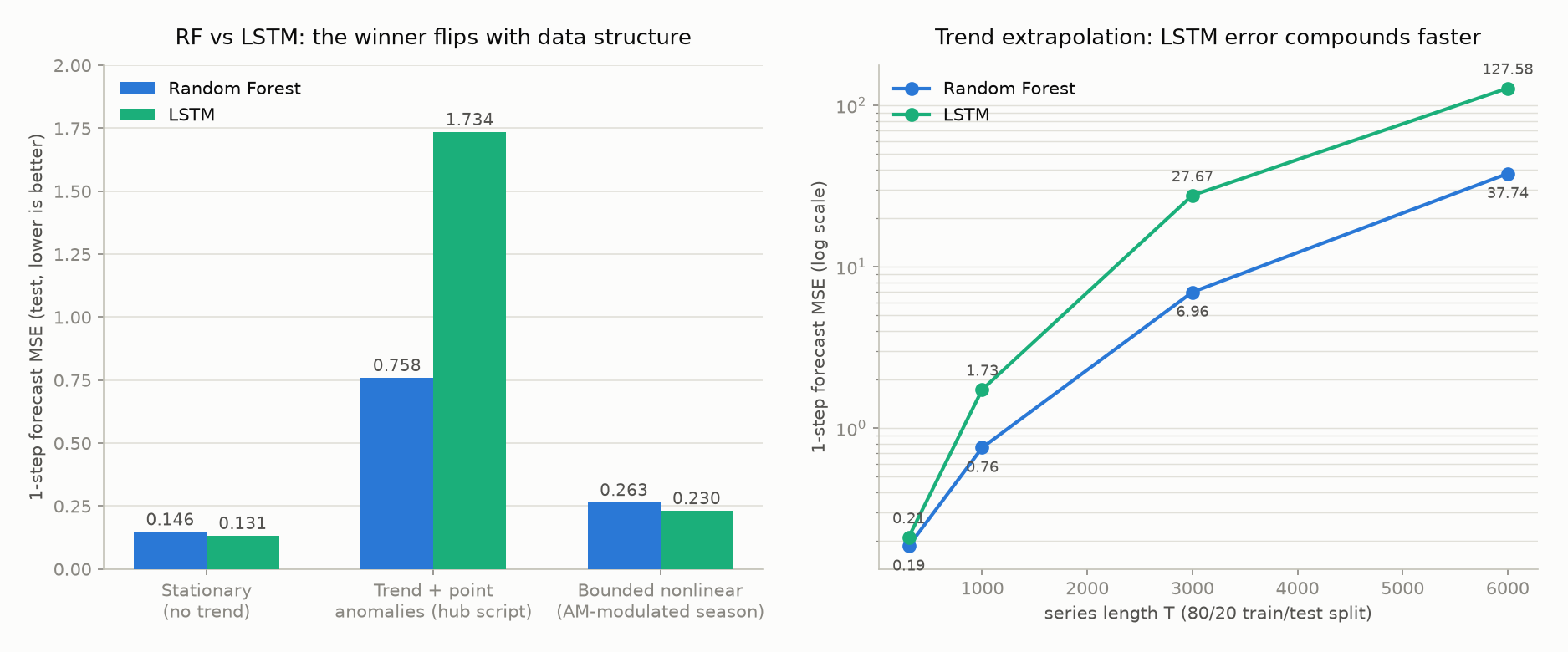
On a stationary series, or a bounded nonlinear structure where the seasonal amplitude is slowly modulated, LSTM edges out RF — its nonlinear gating can capture amplitude-modulation-style interactions. On a series with a trend, however, RF wins clearly. A tree model’s predictions are bounded by the range of values seen in its training leaves, so it “extrapolates poorly but doesn’t blow up,” whereas an LSTM’s recursive state updates let extrapolation error accumulate and amplify over time.
This effect gets more pronounced as the series length \(T\) grows. Sweeping \(T\) from 300 to 6000 on the trending data:
| \(T\) | RF MSE | LSTM MSE | LSTM/RF ratio |
|---|---|---|---|
| 300 | 0.186 | 0.211 | 1.13 |
| 1000 | 0.758 | 1.734 | 2.29 |
| 3000 | 6.958 | 27.673 | 3.98 |
| 6000 | 37.743 | 127.578 | 3.38 |
As \(T\) grows (pushing the test-period trend values further from the training range), both models’ errors grow, but LSTM’s error consistently grows faster than RF’s. The practical takeaway: whichever model you use for a trending series, it is safer to difference the data or remove the trend via STL decomposition before handing it to the forecaster. LSTM in particular carries the risk of nonlinearly ballooning error as the extrapolation range widens.
Recent Research: Tree Models vs. Deep Learning — the Winner Depends on the Regime
The conclusion from this hub’s own experiment — that RF vs. LSTM flips depending on data structure — is corroborated by real-world data. Yang, Gül, and Chen (2025), “Comparative analysis of deep learning and tree-based models in power demand prediction: Accuracy, interpretability, and computational efficiency” (Journal of Building Physics, SAGE), compare tree models (Random Forest / XGBoost / LightGBM) against deep learning (RNN / GRU / LSTM) for power demand forecasting. They report that tree models achieve accuracy roughly on par with deep learning in low-consumption regimes (CV-RMSE 13.62% vs. 12.17%), while deep learning wins in the highly nonlinear, high-consumption peak-demand regime. They also find deep learning’s training time runs 180–369× longer than the tree models’, with tree models also winning on interpretability. This lines up with the direction of this article’s synthetic experiment: which method is optimal depends on whether you are optimizing for accuracy, interpretability, or compute cost.
Around forty lines of code give you five methods times three metrics in one shot. To run it on your own data, swap the synthetic y for your array. Implementation details live in the per-method articles:
k-means / GMM
,
ensembles
,
LSTM
, and
time-series anomaly detection
.
Design Parameter Table
| Method | Key parameters | Recommended starting points |
|---|---|---|
| k-means | number of clusters \(K\) | sweep 2–10 with elbow / silhouette; use n_init=10 to avoid local minima |
| GMM | \(K\) , covariance type | covariance_type: full (flexible) / tied / diag (high-dim) / spherical; minimize BIC |
| Random Forest | n_estimators, max_depth | 200–500 trees, depth 8–20; max_features="sqrt" for classification, 1.0 for regression |
| GBDT | learning_rate, num_leaves, n_estimators | LR 0.05, leaves 31, early stopping for tree count; lower LR × more trees ⇒ higher accuracy |
| LSTM | hidden size \(H\) , layers, lookback | \(H=32\) –\(128\) , 1–2 layers, lookback 1–2× the period; dropout 0.2, Adam LR 1e-3 |
| Kalman filter | process noise \(Q\) , observation noise \(R\) | \(Q/R\) ratio controls tracking; estimate by EM or cross-validation |
| Isolation Forest threshold | contamination | 1–3× the expected anomaly rate; tune by inspecting the score histogram |
Rules of thumb: tree models improve as you lower learning_rate and add more trees (at the cost of compute); LSTM cannot capture seasonality if lookback is below one period and overfits if too high; \(K\)
and layer counts should be chosen mechanically via BIC or validation loss. All of these are amenable to
Bayesian optimization
for automated search.
Related Reading
Entry points for deeper dives from this hub.
The four pillars
- k-means and GMM clustering — hard vs. soft clustering, the EM algorithm
- Ensemble learning (bagging / boosting / stacking) — RF / GBDT / XGBoost / LightGBM
- Time-series forecasting with LSTM — gating, vanishing gradients, Seq2Seq
- Time-series anomaly detection — point vs. sequence anomalies, state-space models
Classical time-series models
- ARIMA and SARIMA time-series forecasting — the linear baseline to benchmark LSTM against
- ARMA/ARIMA in State-Space Form: Kalman-Filter Maximum Likelihood Estimation — derives the Kalman-filter-based exact likelihood that statsmodels’ ARIMA estimation uses internally
- PACF and AR model order identification — identifying the AR order \(p\) with the PACF, the theory behind ARIMA order selection
- GARCH(1,1): Modeling Volatility Clustering — models the variance clustering ARIMA can’t capture via a conditional-variance recursion
- Kalman smoother (RTS) — fixed-interval smoothing for offline accuracy gains
Automated optimization and adjacent tools
- Bayesian optimization for hyperparameter search — directly applicable to GBDT and LSTM tuning
Signal processing hub (twin article)
- Time-frequency analysis hub (FFT / STFT / Wavelet / Hilbert) — feature engineering (spectrogram features) before feeding data into a model
- EMD, VMD, and SSA mode decomposition — decompose non-stationary signals into IMFs as ML features
- Digital Signal Processing and Machine Learning Roadmap — meta path tying the five hubs together
Fifth pillar: Transformer-family time-series models
- Transformer for time-series forecasting: self-attention, positional encoding, Informer — A self-attention-based family that addresses LSTM’s long-range limits, with a lineage Informer → Autoformer → TimesNet. Treat it as the fifth pillar complementing the four core methods above and re-evaluate the LSTM-vs-GBDT trade-offs (sequence length, interpretability, compute) with Transformer added to the table.
Conclusion
When applying machine learning to time-series, classification, or anomaly tasks, the cleanest path is: narrow down by the three axes supervised/unsupervised × sequential dependence × interpretability, sanity-check against sample size and compute in the feature matrix, and start from whichever decision scenario most closely matches your problem.
- Unlabeled, looking for groups → k-means / GMM
- Tabular classification or short–medium horizon forecasting with interpretability → Random Forest / GBDT
- Long-range dependence and nonlinearity → LSTM
- Sequence anomalies or state tracking → Kalman filter family / LSTM-AE
- Automatic hyperparameter search → Bayesian optimization
When in doubt, copy the unified Python evaluation script in this article, swap in your own data, and read MSE / F1 / silhouette across the five methods. From here, the next themes worth deepening are (a) Gaussian process regression for small-data forecasting with calibrated intervals, (b) Transformer-family time-series models (Informer, TimesNet), (c) deep state-space models that mix neural networks with state-space structure, and (d) the bridge to causal inference, where feature importance becomes intervention effect. Use this hub and the linked articles as a two-way map for finding the right tool for your problem.