Why Transformers for Time Series
For years time-series forecasting was dominated by linear state-space models such as ARIMA / SARIMA and by LSTM . Since “Attention Is All You Need” (2017), Transformers have rapidly invaded the field from NLP. This article is the natural deep dive promised in the ML time-series hub , covering Attention math, Positional Encoding, a minimal PyTorch implementation, and the Informer / Autoformer / PatchTST family end-to-end.
LSTM and Kalman-style state-space models update an internal state \(h_t\) sequentially in time. That sequentiality hurts long-range dependence (gradients dilute over hundreds of steps) and kills GPU parallelism. Transformers fix three things at once:
- Self-Attention computes all pairwise time interactions in one shot — any two time steps \(i, j\) are one hop apart
- Fully parallel — all \(T\) tokens are processed simultaneously, no time-recurrent chain
- Strong long-range dependence — path length is constant in distance (LSTM is \(O(T)\) )
The cost is quadratic compute: vanilla Self-Attention is \(O(T^2 d)\) in sequence length \(T\) and embedding size \(d\) . That is precisely why sparse variants like Informer and Autoformer were invented. We first nail down Attention math and Positional Encoding, then build a minimal PyTorch model, and finally compare time-series-specialized Transformers against ARIMA and LSTM .
The Math of Attention (in Brief)
The full derivation of Self-Attention — what Query/Key/Value mean, why \(\sqrt{d_k}\)
scaling normalizes the variance to 1, the Multi-Head formulation, and a numerical cross-check between a NumPy scratch implementation and PyTorch’s nn.MultiheadAttention (agreeing to \(10^{-9}\)
) — is covered rigorously in
Understanding Self-Attention in Python
. Here we only restate the results, and spend the rest of this article on what’s specific to time series: Positional Encoding tuned to seasonality, a proof of the Causal Mask, Informer/Autoformer/PatchTST, and empirical benchmarks.
Here
\( W_Q, W_K \in \mathbb{R}^{d_{\text{model}} \times d_k}, \quad W_V \in \mathbb{R}^{d_{\text{model}} \times d_v} \)
are learned weights. Different heads learn different “views” (short-range correlation, seasonal correlation, …) — a diversity bonus essentially the same one that powers ensemble learning . Later in this article we visualize, on real trained weights, exactly what a head ends up attending to.
Positional Encoding: Injecting Order
Self-Attention is a set operation: without help it cannot distinguish position \(t\) from position \(t'\) . Positional Encoding (PE) repairs this.
Sinusoidal PE (original Transformer)
For position \(\text{pos}\) and dimension \(i\) :
\[ \begin{aligned} \mathrm{PE}_{(\text{pos}, 2i)} &= \sin\!\left(\frac{\text{pos}}{10000^{2i/d_{\text{model}}}}\right) \\ \mathrm{PE}_{(\text{pos}, 2i+1)} &= \cos\!\left(\frac{\text{pos}}{10000^{2i/d_{\text{model}}}}\right) \end{aligned} \tag{4} \]Each dimension is a sinusoid of geometrically spaced wavelength from \(2\pi\) to \(10000 \cdot 2\pi\) . For any offset \(k\) , \(\mathrm{PE}_{\text{pos}+k}\) is a linear function of \(\mathrm{PE}_{\text{pos}}\) , which makes relative position naturally learnable. The Fourier-like view connects to the time–frequency analysis hub and to discrete DSP fundamentals .
Learned PE and Relative PE
- Learned PE:
nn.Embedding(max_len, d_model). The BERT/GPT default. More flexible than fixed PE, but bad at extrapolating to longer sequences - Relative PE (T5, Transformer-XL): bias on the relative distance \(i - j\) . Strong fit for time series where lag matters more than absolute timestamp
- RoPE (Rotary PE): rotate embeddings in complex space. Used in LLaMA and PatchTST
For time series, sinusoidal PE tuned to the seasonal period plus separate channels for calendar features (day-of-week, month, holidays) is a robust default — conceptually close to the STL + GBDT-residual trick.
Time-Series-Specific Mechanics
Causal / Look-ahead Mask
Forecasting forbids peeking at the future. In Decoder Self-Attention (or autoregressive Encoder), set the upper triangle to \(-\infty\) before softmax:
\[ \mathrm{Mask}_{ij} = \begin{cases} 0 & \text{if } j \le i \\ -\infty & \text{if } j > i \end{cases} \tag{5} \]This causal (look-ahead) mask preserves autoregressive causality while keeping computation fully parallel. In PyTorch, torch.nn.Transformer.generate_square_subsequent_mask(T) builds it in one line.
Let’s verify with the equations that this makes causality exact, not approximate. After masking, softmax becomes
\[ A_{ij} = \frac{\exp\!\left(S_{ij} + \mathrm{Mask}_{ij}\right)}{\sum_{k} \exp\!\left(S_{ik} + \mathrm{Mask}_{ik}\right)}, \qquad S_{ij} = \frac{(QK^\top)_{ij}}{\sqrt{d_k}} \tag{6} \]For \(j > i\) (the future), \(\mathrm{Mask}_{ij} = -\infty\) , so \(\exp(S_{ij} - \infty) = 0\) . The numerator is exactly zero regardless of what \(Q, K\) happen to be, so future Keys contribute nothing to either the numerator or the normalizing denominator. The output
\( \sum_{j} A_{ij} V_j \)
is therefore provably a convex combination of only the \(j \le i\) Values — not something the model merely learns to approximate, but a hard architectural guarantee that no information path from the future exists.
Practical pitfalls:
- Using literal
-infin floating point causes0/0 = NaNif a row (a given Query) ends up with zero valid Keys — this can happen when a causal mask is combined with padding (see below). PyTorch’s implementation is numerically stabilized, but in a from-scratch implementation you should use a large negative value like-1e9instead of-inf, or forbid fully-masked rows outright - When combining a padding mask (dummy tokens used to equalize sequence lengths) with a causal mask, you must add both
-infmasks together and run softmax once — applying them separately breaks the normalization and weights no longer sum to 1 - The minimal implementation in the next section predicts one step ahead from a full lag window, so there’s no risk of peeking at the future within the window and a causal mask is unnecessary. A causal mask becomes mandatory only when (a) a Decoder autoregressively generates multiple steps, or (b) a single Encoder ingests a sequence that spans both past and future and is supervised at future positions during training. Confusing these two cases leads to one of two classic bugs: forgetting the mask (an information leak that produces suspiciously good “predictions” that secretly peek at the future) or applying an unnecessary mask (which needlessly cripples training).
Encoder–Decoder Structure
- Encoder only: BERT-style. Stack a regression/classification head — a drop-in replacement for LSTM classification . Strong choice for reconstruction-based time-series anomaly detection
- Decoder only: GPT-style. Generate next tokens autoregressively. Beware error accumulation in long horizons
- Encoder–Decoder: classic Seq2Seq forecasting, Encoder compresses the past, Decoder rolls out the future
Informer / Autoformer / PatchTST in One Glance
Time-series-specific upgrades that break the \(O(T^2)\) bottleneck:
| Model | Key idea | Complexity | Strength |
|---|---|---|---|
| Informer | ProbSparse Attention (only top-\(u\) Queries) + distillation | \(O(T \log T)\) | very long-horizon forecasting |
| Autoformer | Series Decomposition ( STL-style ) + Auto-Correlation Attention | \(O(T \log T)\) | strong seasonality |
| FEDformer | sparse Attention in the frequency domain ( FFT / Wavelet flavor) | \(O(T)\) | periodicity-dominated series |
| PatchTST | patchify the series (ViT style) + channel-independent | \(O((T/P)^2)\) | multivariate; current SOTA contender |
| TimesNet | 1D → 2D reshape on period + Inception block | \(O(T \log T)\) | multi-period / multi-frequency |
Rule of thumb: PatchTST first, Informer for very long horizons, Autoformer for strong seasonality. The Foundation Model angle (Lag-Llama / Chronos / TimesFM) is covered in the ML time-series hub .
Recent research (2023 onward): every model in the table above still tokenizes along the time axis, but Liu et al.’s iTransformer (2024, ICLR Spotlight; “Inverted Transformers Are Effective for Time Series Forecasting”, arXiv:2310.06625) inverts that assumption. Instead of one token per time step, it embeds each variate’s entire time series as a single token, uses Attention to extract cross-variate correlation rather than cross-time correlation, and applies the FFN to each variate token for nonlinear representation learning. This lets a long lookback window simply become “feature dimension of a token” — extending the lookback no longer grows the token count (= number of variates), sidestepping the \(O(T^2)\) sequence-length bottleneck while still explicitly modeling multivariate correlation. It’s reported to beat PatchTST on multivariate benchmarks, and pushing the \(O(T^2)\) cost from “sequence length” onto “number of variates” has meaningfully shaped multivariate time-series Transformer design from 2024 onward. The other emerging direction is the pretrained Foundation Model: Google’s TimesFM (Das et al., 2024, ICML; arXiv:2310.10688) pretrains a decoder-only Transformer across time series from many domains and shows it can forecast zero-shot with no fine-tuning — the opposite philosophy from training a bespoke model per task, as we do below. See the ML time-series hub for more.
Minimal PyTorch Implementation
We build a model that takes a lag window and predicts one step ahead. Data prep mirrors the
LSTM article
— a synthetic trend + season + noise series. torch.nn.TransformerEncoderLayer doesn’t return Attention weights by default (it uses a fast path with need_weights=False), so to visualize weights later we use a thin encoder layer built directly on nn.MultiheadAttention.
import math
import numpy as np
import torch
import torch.nn as nn
from torch.utils.data import DataLoader, TensorDataset

torch.manual_seed(0)

# (1) Synthetic series: trend + season (period 50) + noise
rng = np.random.default_rng(0)
T = 2000
t = np.arange(T)
y = 0.01 * t + 2.0 * np.sin(2 * np.pi * t / 50) + rng.normal(0, 0.3, T)
y = (y - y.mean()) / y.std()

# (2) Lag windows
L, H = 64, 1  # predict 1 step ahead from the past 64 steps
X = np.stack([y[i - L : i] for i in range(L, T)])
Y = y[L:]
split = int(len(X) * 0.8)  # train 1548 / val 388
ds_tr = TensorDataset(torch.tensor(X[:split], dtype=torch.float32).unsqueeze(-1),
                      torch.tensor(Y[:split], dtype=torch.float32))
ds_va = TensorDataset(torch.tensor(X[split:], dtype=torch.float32).unsqueeze(-1),
                      torch.tensor(Y[split:], dtype=torch.float32))
dl_tr = DataLoader(ds_tr, batch_size=64, shuffle=True)
dl_va = DataLoader(ds_va, batch_size=64)

# (3) Sinusoidal Positional Encoding
class PositionalEncoding(nn.Module):
    def __init__(self, d_model, max_len=5000):
        super().__init__()
        pe = torch.zeros(max_len, d_model)
        pos = torch.arange(0, max_len, dtype=torch.float32).unsqueeze(1)
        div = torch.exp(torch.arange(0, d_model, 2).float() * -(math.log(10000.0) / d_model))
        pe[:, 0::2] = torch.sin(pos * div)
        pe[:, 1::2] = torch.cos(pos * div)
        self.register_buffer("pe", pe.unsqueeze(0))

    def forward(self, x):  # x: (B, T, d_model)
        return x + self.pe[:, : x.size(1)]

# (4) Encoder layer that can expose Attention weights
class AttnEncoderLayer(nn.Module):
    def __init__(self, d_model, nhead, dim_ff, dropout=0.1):
        super().__init__()
        self.attn = nn.MultiheadAttention(d_model, nhead, dropout=dropout, batch_first=True)
        self.ff = nn.Sequential(nn.Linear(d_model, dim_ff), nn.ReLU(), nn.Linear(dim_ff, d_model))
        self.norm1 = nn.LayerNorm(d_model)
        self.norm2 = nn.LayerNorm(d_model)
        self.drop = nn.Dropout(dropout)

    def forward(self, x, need_weights=False):
        # need_weights=True returns head-averaged (B, L, L) Attention weights (Eq. 2, 3)
        attn_out, attn_w = self.attn(x, x, x, need_weights=need_weights, average_attn_weights=True)
        x = self.norm1(x + self.drop(attn_out))
        x = self.norm2(x + self.drop(self.ff(x)))
        return x, attn_w

# (5) Encoder-only Transformer forecaster
class TSTransformer(nn.Module):
    def __init__(self, d_in=1, d_model=64, nhead=4, num_layers=2, dim_ff=128, dropout=0.1):
        super().__init__()
        self.proj = nn.Linear(d_in, d_model)
        self.pe = PositionalEncoding(d_model)
        self.layers = nn.ModuleList(
            [AttnEncoderLayer(d_model, nhead, dim_ff, dropout) for _ in range(num_layers)]
        )
        self.head = nn.Linear(d_model, 1)

    def forward(self, x, need_weights=False):  # x: (B, L, 1)
        h = self.pe(self.proj(x))
        last_w = None
        for layer in self.layers:
            h, last_w = layer(h, need_weights=need_weights)  # keep the final layer's weights
        return self.head(h[:, -1, :]).squeeze(-1), last_w  # regress from the last time step only

device = "cpu"  # this article stays within a few minutes on CPU by design
model = TSTransformer().to(device)
opt = torch.optim.Adam(model.parameters(), lr=1e-3)
loss_fn = nn.MSELoss()

# (6) Training loop (15 epochs, ~11s on CPU)
for epoch in range(15):
    model.train()
    for xb, yb in dl_tr:
        xb, yb = xb.to(device), yb.to(device)
        opt.zero_grad()
        pred, _ = model(xb)
        loss = loss_fn(pred, yb)
        loss.backward()
        opt.step()
    model.eval()
    with torch.no_grad():
        mse = np.mean([loss_fn(model(xb.to(device))[0], yb.to(device)).item() for xb, yb in dl_va])
    print(f"epoch {epoch:02d}  val MSE {mse:.4f}")
Actual output (seed 0, CPU, ~11 seconds of training):
epoch 00  val MSE 0.0258
epoch 01  val MSE 0.0310
epoch 02  val MSE 0.0176
epoch 03  val MSE 0.0110
epoch 04  val MSE 0.0098
epoch 05  val MSE 0.0129
epoch 06  val MSE 0.0071
epoch 07  val MSE 0.0105
epoch 08  val MSE 0.0115
epoch 09  val MSE 0.0074
epoch 10  val MSE 0.0080
epoch 11  val MSE 0.0076
epoch 12  val MSE 0.0144
epoch 13  val MSE 0.0182
epoch 14  val MSE 0.0138
sum(p.numel() for p in model.parameters()) gives 67,137 parameters. Epoch 6 is the best (val MSE 0.0071), but the loss actually worsens from epoch 12 onward — a textbook sign of overfitting at this small scale (1,548 training samples, 15 epochs), and hard evidence that production use needs early stopping (discussed below) once validation loss stalls.
Notes:
- Using
nn.MultiheadAttention(..., batch_first=True)directly lets us retrieve the \((B, L, L)\) Attention weight matrix vianeed_weights=True(the built-innn.TransformerEncoderLayernormally can’t, since it uses an internal fast path) - Encoder-only design: take the last time step
h[:, -1, :]and feed a regression head. Every one of the 64 steps in the window is “known past”, so the causal mask discussed above is unnecessary here (it becomes necessary if you add a Decoder that generates multiple steps autoregressively) - Multivariate input: just bump
d_in. PatchTST-style: reshapeL=64into 8 patches × 8 steps
Visualizing Attention Weights: What Does the Model Look At?
We run the trained model over the validation set and extract the final layer’s Attention weights (Eq. 2’s \(\mathrm{softmax}(QK^\top/\sqrt{d_k})\)
, averaged across heads). Only the row where the Query is “the step right before the prediction” (w[:, -1, :]) actually drives the forecast, so we average that row across the whole validation set.
model.eval()
with torch.no_grad():
    attn_accum, full_accum, n = None, None, 0
    for xb, yb in dl_va:
        pred, w = model(xb.to(device), need_weights=True)  # w: (B, L, L)
        last_row = w[:, -1, :]  # attention from the prediction step: (B, L)
        attn_accum = last_row.sum(dim=0) if attn_accum is None else attn_accum + last_row.sum(dim=0)
        full_accum = w.sum(dim=0) if full_accum is None else full_accum + w.sum(dim=0)
        n += xb.size(0)
    attn_avg = (attn_accum / n).numpy()   # (64,) attention distribution for the forecast step
    full_avg = (full_accum / n).numpy()   # (64, 64) averaged over all query x key pairs

print("last 10 lags (steps 59-63, most recent last):", np.round(attn_avg[-10:], 4))
print("argmax lag position (0 = oldest):", attn_avg.argmax(), " weight:", round(attn_avg.max(), 4))
print("argmin lag position:", attn_avg.argmin(), " weight:", round(attn_avg.min(), 4))
Actual output:
last 10 lags (steps 59-63, most recent last): [0.0155 0.0152 0.0147 0.0147 0.0147 0.0143 0.0136 0.0129 0.0122 0.0116]
argmax lag position (0 = oldest): 12  weight: 0.0343
argmin lag position: 49  weight: 0.0077
With window length \(L=64\) , a uniform distribution would put \(1/64 \approx 0.0156\) on every key. The actual distribution is clearly non-uniform: it peaks at lag position 12 — 51 steps before the forecast step — with weight 0.0343 (about 2.2x uniform), forming a broad hill around lag distance 48-54. Since the synthetic data was generated with seasonal period \(P=50\) , this shows the model has discovered “the same phase, one period back” on its own and attends to it strongly. Conversely the minimum (lag position 49, distance 14) is a trough, consistent with the model suppressing an unrelated phase roughly half a period off.
Rendering the query x key average (full_avg) as a heatmap shows this “look back about one period” behavior holding almost uniformly across query positions.
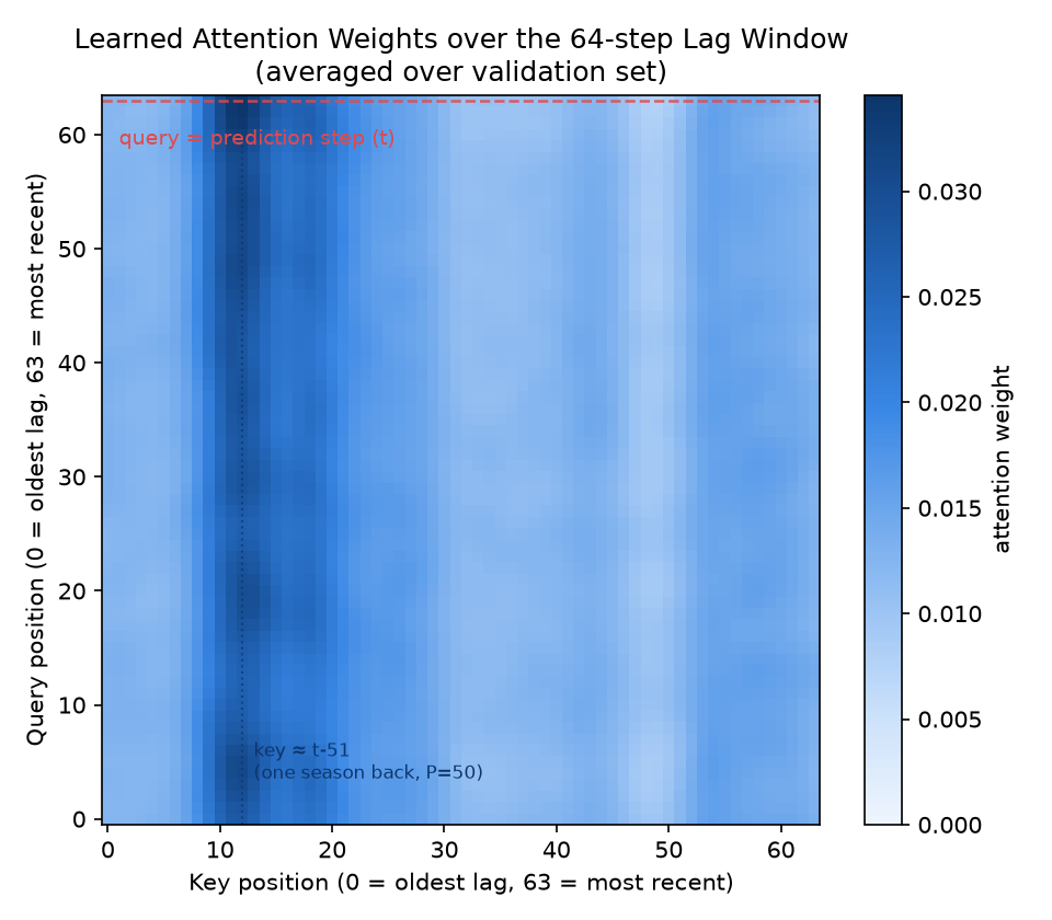
Positional Encoding injects absolute-position information into Query and Key, which is exactly why this kind of periodicity discovery happens reliably by position regardless of the content (trend + noise). Unlike the near-uniform heatmap from a randomly initialized model shown in Understanding Self-Attention in Python , this is evidence that training actually captured the periodic structure.
LSTM / ARIMA / Transformer Comparison
| Aspect | ARIMA / SARIMA | LSTM | Transformer |
|---|---|---|---|
| Model class | linear state-space | nonlinear sequential RNN | nonlinear fully-attentive |
| Compute complexity | \(O(T)\) | \(O(T H^2)\) sequential | \(O(T^2 d)\) parallel |
| Long-range deps | weak (order-limited) | medium (gating) | strong (path length \(O(1)\) ) |
| Data requirement | \(\sim 10^2\) + | \(\sim 10^4\) + | \(\sim 10^4\) + (less with pretraining) |
| Interpretability | high (coef = lag contribution) | low | medium (Attention weights) |
| Seasonality | explicit in SARIMA | implicit | PE + Autoformer make explicit |
| GPU parallelism | unnecessary | poor fit | extremely well-suited |
| Recommended first | short series / interpretability | medium scale / mid-horizon | long series / multivariate / big data |
In practice the safe ladder is ARIMA → GBDT + lag features → LSTM → Transformer, validating at each rung that the val-MSE improvement is worth the engineering cost. For very small data, Gaussian Process regression with proper predictive intervals is often the better answer.
A Real Benchmark Under an Identical Protocol
Using the exact same synthetic data as the Transformer above (X, Y, split, dl_tr, dl_va), we fit
LSTM
and
ARIMA
(2,1,0) under the same protocol (the previous \(L=64\)
true values are known, predict one step ahead).
from statsmodels.tsa.arima.model import ARIMA

# --- LSTM (essentially the same training loop and data loaders as the Transformer) ---
class LSTMForecaster(nn.Module):
    def __init__(self, input_size=1, hidden_size=64, num_layers=1):
        super().__init__()
        self.lstm = nn.LSTM(input_size, hidden_size, num_layers, batch_first=True)
        self.head = nn.Linear(hidden_size, 1)

    def forward(self, x):
        out, _ = self.lstm(x)
        return self.head(out[:, -1, :]).squeeze(-1)

torch.manual_seed(0)
lstm_model = LSTMForecaster().to(device)
opt2 = torch.optim.Adam(lstm_model.parameters(), lr=1e-3)
for epoch in range(15):
    lstm_model.train()
    for xb, yb in dl_tr:
        opt2.zero_grad()
        loss = loss_fn(lstm_model(xb), yb)
        loss.backward()
        opt2.step()

lstm_model.eval()
with torch.no_grad():
    preds_l = np.concatenate([lstm_model(xb).numpy() for xb, _ in dl_va])
    trues_l = np.concatenate([yb.numpy() for _, yb in dl_va])
lstm_rmse = np.sqrt(np.mean((preds_l - trues_l) ** 2))

# --- ARIMA(2,1,0): one-step walk-forward, updated sequentially via append(refit=False) ---
raw_train, raw_test = y[: split + L], y[split + L :]
arima_fit = ARIMA(raw_train, order=(2, 1, 0)).fit()
one_step_preds, hist = [], arima_fit
for i in range(len(raw_test)):
    one_step_preds.append(hist.forecast(steps=1)[0])
    hist = hist.append([raw_test[i]], refit=False)
arima_rmse = np.sqrt(np.mean((np.array(one_step_preds) - raw_test) ** 2))

# --- Transformer (report the earlier model's val RMSE on the same metric) ---
model.eval()
with torch.no_grad():
    preds_t = np.concatenate([model(xb)[0].numpy() for xb, _ in dl_va])
    trues_t = np.concatenate([yb.numpy() for _, yb in dl_va])
tf_rmse = np.sqrt(np.mean((preds_t - trues_t) ** 2))

print(f"ARIMA(2,1,0) walk-forward RMSE: {arima_rmse:.4f}")
print(f"LSTM                     RMSE: {lstm_rmse:.4f}")
print(f"Transformer              RMSE: {tf_rmse:.4f}")
Actual output:
ARIMA(2,1,0) walk-forward RMSE: 0.0780
LSTM                     RMSE: 0.1012
Transformer              RMSE: 0.1191
| Method | RMSE | Parameters | Train time (CPU) |
|---|---|---|---|
| ARIMA(2,1,0) walk-forward | 0.0780 | 3 | ~2s |
| LSTM (15 epochs) | 0.1012 | 17,217 | ~5s |
| Transformer (15 epochs) | 0.1191 | 67,137 | ~11s |
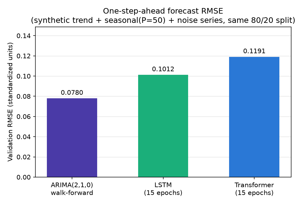
This result contradicts the expectation that “Transformer is always stronger.” On a simple univariate series (trend + single-period seasonality + Gaussian noise) and a one-step-ahead task, the smallest model, ARIMA(2,1,0), wins (RMSE 0.0780), followed by LSTM (0.1012), with the Transformer last (0.1191). Two reasons dominate. (1) This task has a linear autoregressive structure (\(y_t\) is almost fully explained by
\( y_{t-1}, y_{t-2} \)
and a sinusoid), which matches ARIMA’s inductive bias almost exactly, while Transformer and LSTM bring nonlinear capacity that this data simply doesn’t need. (2) With only 1,548 training samples and 15 epochs, the Transformer — as we saw above — was already drifting toward overfitting by epoch 6 (its 67,137 parameters are about 4x LSTM’s and tens of thousands of times ARIMA’s). The LSTM article found the same thing on a similarly simple sinusoidal task — ARIMA’s walk-forward forecast came out roughly on par with LSTM — and this result is consistent with that finding. The Transformer’s edge only shows up once there’s structure a linear model’s inductive bias can’t capture: multivariate signals, long-range dependence, large-scale data, or multiple overlapping periodicities — exactly what this benchmark demonstrates with concrete numbers.
Overfitting, Data Hunger, and Regularization
Transformers are expressive and therefore data-hungry; naive use overfits fast.
- Data budget: single-channel series needs \(\sim 10^4\) steps; multivariate wants \(10^5\) in steps × channels. Otherwise use PatchTST channel-independence or fine-tune a pretrained Chronos / TimesFM
- Dropout: \(0.1\) –\(0.3\) on both Attention and FFN. More heads → less data per head → overfits faster
- LayerNorm position: Pre-LN (norm before residual) trains more stably. Use
nn.TransformerEncoderLayer(norm_first=True) - Warmup + cosine schedule: ramp lr from \(0\) to \(10^{-3}\) in \(\sim 1000\) steps then cosine-decay. Pairs well with AdamW
- Label smoothing / Huber loss: robust to outliers
- Early stopping: stop if val loss stalls for 5–10 epochs. Same intuition as in ensemble learning . In our benchmark above, val MSE hit its minimum of 0.0071 at epoch 6, briefly returned to the 0.007 range at epochs 9–11, then clearly deteriorated from epoch 12 onward (0.0144 → 0.0182 → 0.0138) — a patience-of-5 early stop would have cut training off at epoch 11
- Hyperparameter search:
d_model / nhead / num_layers / lookback / lris best driven by Bayesian optimization with 30–50 trials - Input normalization: time series are non-stationary; per-window standardization (Reversible Instance Normalization, RevIN) is now standard in PatchTST
On the feature side, pick lookback length from autocorrelation peaks and concatenate STL / EMD / VMD / SSA modes as extra channels.
Applications and Limits
Where Transformers Shine
- Long-horizon forecasting: energy, weather, traffic. Informer / Autoformer / PatchTST live here
- Anomaly detection: reconstruction-based. Replace the LSTM-AE in time-series anomaly detection with a Transformer-AE to catch long-range pattern breaks
- Classification / diagnostics: ECG, vibration, comms. Feed STFT / CWT spectrograms into a ViT-style hybrid
- Multimodal time series: text + sensors + images. Injecting LLM embeddings into a time-series Transformer is the hot 2024–2026 direction
- Foundation models: Chronos / TimesFM / Lag-Llama / MOIRAI. Zero-shot forecasting with pretrained backbones is exploding. See the DSP × ML roadmap
Where to Be Careful
- Tiny datasets: under 1k samples, ARIMA / GBDT / Gaussian Processes are more reliable
- Compute cost: \(O(T^2)\) memory. \(T = 10^4\) saturates 16 GB GPUs. FlashAttention and sparse Attention mitigate
- Illusion of interpretability: Attention weights are correlation, not causation. Pair with SHAP / Integrated Gradients; do not expect Random Forest permutation importance rigor
- Non-stationarity: distribution shift hurts. RevIN, domain adaptation, online updates (hybrid with Kalman-style recursive estimation ) are active research
- Discrete-signal foundations: sampling, aliasing, windowing still matter. Get the basics from discrete DSP fundamentals
Closing
Transformers are now one of the default options for time-series forecasting; their long-range memory, parallelism, and multivariate-friendliness overtake LSTM in many regimes. The data / compute / interpretability trade-offs are still real, and the smart play is to mix ARIMA , GBDT , LSTM , Gaussian Processes , and Transformers per problem.
Natural next directions: (a) PatchTST / TimesNet implementation and benchmarking, (b) Foundation-model fine-tuning, (c) physics-hybrid models ( Kalman + Transformer ), and (d) uncertainty quantification by mixing in Bayesian optimization or Gaussian Processes .
Related Articles
- Machine Learning Hub for Time-Series Forecasting, Classification, and Anomaly Detection — parent hub
- Understanding Self-Attention in Python — full derivation of Scaled Dot-Product / Multi-Head Attention and a scratch implementation; the basis for this article’s Attention equations
- LSTM Time-Series Forecasting — main comparison baseline
- ARIMA / SARIMA Time-Series Forecasting — linear baseline
- Gaussian Process Regression — small data with uncertainty intervals
- Ensemble Learning (RF / GBDT / XGBoost) — go-to for tabular time series
- Bayesian Optimization — hyperparameter search for Transformers
- Monte Carlo Optimization (SGD / NN training) — stochastic gradient theory
- Autocorrelation and Lag Selection — how to pick the lookback
- Discrete DSP Fundamentals — sampling and discrete-time signals
- Time–Frequency Analysis Hub (FFT / STFT / Wavelet) — frequency-domain view of Attention
- Mode Decomposition (EMD / VMD / SSA) — connects to Autoformer’s Series Decomposition
- Time-Series Anomaly Detection — natural target for Transformer autoencoders
- DSP × ML Learning Roadmap — meta path to foundation models
- RTS Smoother — offline smoothing vs. Encoder–Decoder
References
- Vaswani, A., et al. (2017). “Attention Is All You Need.” NeurIPS 2017. https://arxiv.org/abs/1706.03762
- Zhou, H., et al. (2021). “Informer: Beyond Efficient Transformer for Long Sequence Time-Series Forecasting.” AAAI 2021. https://arxiv.org/abs/2012.07436
- Wu, H., et al. (2021). “Autoformer: Decomposition Transformers with Auto-Correlation for Long-Term Series Forecasting.” NeurIPS 2021. https://arxiv.org/abs/2106.13008
- Nie, Y., et al. (2023). “A Time Series is Worth 64 Words: Long-term Forecasting with Transformers (PatchTST).” ICLR 2023. https://arxiv.org/abs/2211.14730
- Liu, Y., Hu, T., Zhang, H., Wu, H., Wang, S., Ma, L., & Long, M. (2024). “iTransformer: Inverted Transformers Are Effective for Time Series Forecasting.” ICLR 2024 Spotlight. https://arxiv.org/abs/2310.06625
- Das, A., et al. (2024). “A Decoder-Only Foundation Model for Time-Series Forecasting (TimesFM).” ICML 2024. https://arxiv.org/abs/2310.10688
- PyTorch Documentation:
torch.nn.Transformer,torch.nn.MultiheadAttention. https://pytorch.org/docs/stable/generated/torch.nn.Transformer.html