Introduction
The Nyquist-Shannon sampling theorem guarantees that a band-limited signal can be perfectly reconstructed if it is sampled above the Nyquist rate. In practical systems, however, we frequently need to change the sampling rate in the middle of a processing chain:
- Audio format conversion: CD (44.1 kHz) ↔ professional audio and video (48 kHz)
- Delta-sigma ADCs: decimating a 1-bit stream oversampled at several MHz down to tens of kHz
- Communication systems: matching symbol rates to DAC/ADC rates, pulse shaping
- Wavelet transforms and filter banks: the structure itself downsamples by 2 at every stage
The discipline that handles systems with multiple coexisting sampling rates is multirate signal processing. This article systematically covers the frequency-domain behavior of downsampling (decimation) and upsampling (interpolation), rational-rate resampling, and the two ideas that make it all computationally efficient — polyphase decomposition and the Noble identities — with mathematical derivations and Python implementations using scipy.signal.decimate, resample, resample_poly, and upfirdn.
For the big picture of discrete-time signal processing, see the Discrete Signal Processing Fundamentals Roadmap ; for the continuous-time side of interpolation, see Signal Reconstruction and Interpolation .
Downsampling (Decimation)
Definition and Frequency-Domain Analysis
Keeping only every \(M\) -th sample of a signal \(x[n]\) (downsampling by \(M\) ) is defined as:
\[y[m] = x[Mm] \tag{1}\]The sampling rate drops from \(f_s\) to \(f_s / M\) . In the DTFT domain, the spectrum is stretched by a factor of \(M\) and \(M\) shifted copies are superimposed:
\[Y(e^{j\omega}) = \frac{1}{M} \sum_{k=0}^{M-1} X\!\left(e^{j(\omega - 2\pi k)/M}\right) \tag{2}\]The \(k = 0\) term is the desired (stretched) spectrum; the \(k \neq 0\) terms are aliasing components. If the original signal is band-limited to \(|\omega| < \pi / M\) (i.e., \(f < f_s / 2M\) in physical frequency), the copies do not overlap and no aliasing occurs.
Why an Anti-Aliasing Filter Is Mandatory
Real signals usually contain energy above \(\pi / M\) , so a low-pass filter with cutoff \(\pi / M\) must precede the downsampler. The combination “LPF + downsampler” is called decimation:
\[y[m] = \sum_{k} h[k] \, x[Mm - k] \tag{3}\]where \(h[n]\) is the impulse response of the anti-aliasing filter. For the fundamentals of filter design, see Low-Pass Filter Design and Comparison and FIR vs IIR Filters .
Python: Naive Downsampling vs scipy.signal.decimate
scipy.signal.decimate bundles the anti-aliasing filter and the downsampler. Comparing it with naive slicing x[::M] makes the aliasing visible.
import numpy as np
import matplotlib.pyplot as plt
from scipy.signal import decimate
# --- Test signal: desired 50 Hz component + 380 Hz high-frequency component ---
fs = 1000 # original sampling rate [Hz]
t = np.arange(0, 2.0, 1/fs)
x = np.sin(2*np.pi*50*t) + 0.8*np.sin(2*np.pi*380*t)
M = 4 # decimation factor: 1000 Hz -> 250 Hz (new Nyquist 125 Hz)
fs_new = fs / M
# (1) Naive slicing without a filter -> 380 Hz aliases down to 120 Hz
x_naive = x[::M]
# (2) decimate: anti-aliasing filter + downsampling
x_dec = decimate(x, M, ftype='fir', zero_phase=True)
def spectrum_db(sig, fs):
"""Hann-windowed magnitude spectrum in dB (normalized to the maximum)."""
win = np.hanning(len(sig))
X = np.abs(np.fft.rfft(sig * win))
f = np.fft.rfftfreq(len(sig), 1/fs)
return f, 20*np.log10(X / X.max() + 1e-12)
fig, axes = plt.subplots(3, 1, figsize=(10, 9), sharex=False)
f0, S0 = spectrum_db(x, fs)
axes[0].plot(f0, S0)
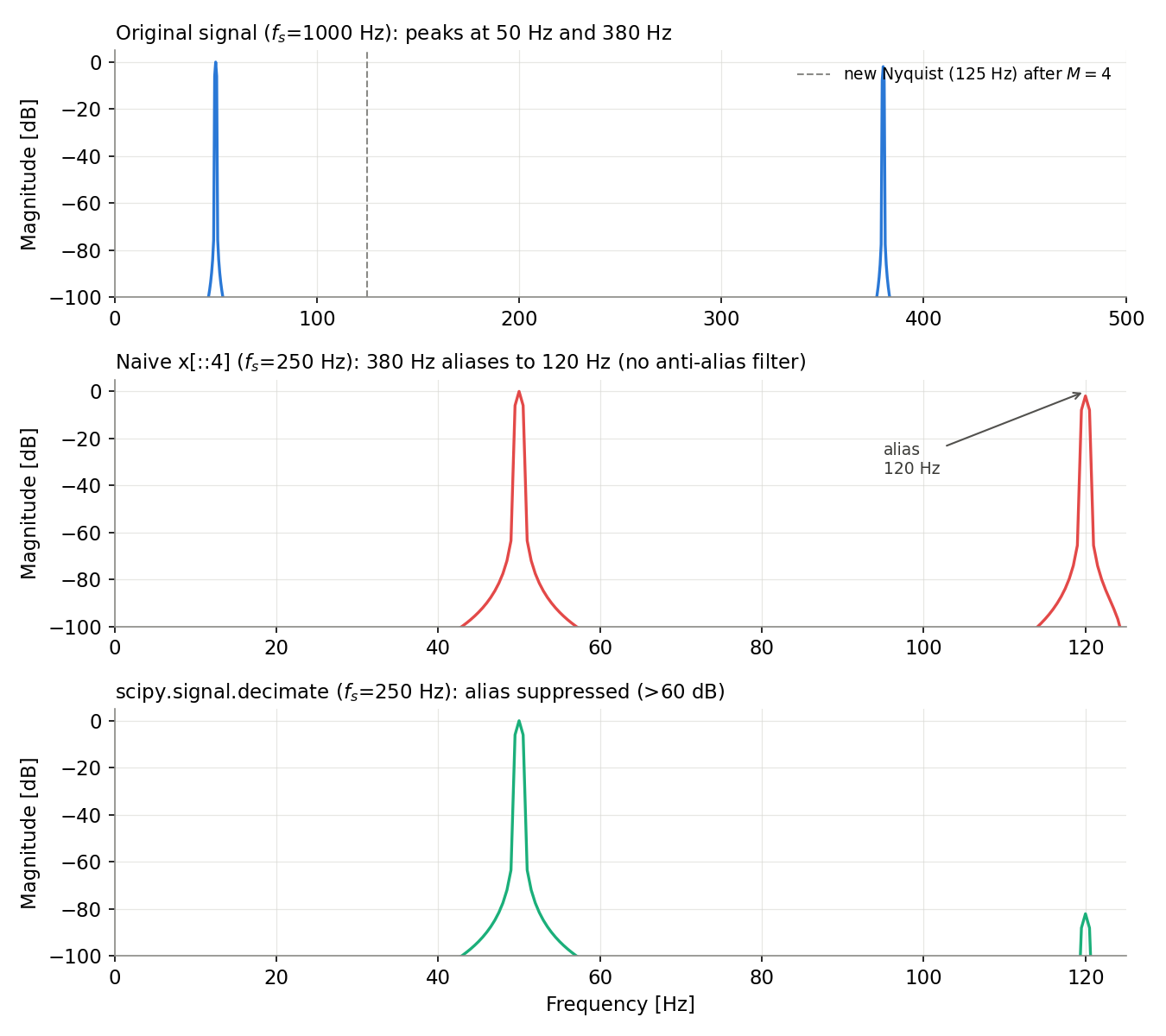
axes[0].set_title('Original (fs=1000 Hz): peaks at 50 Hz and 380 Hz')
axes[0].set_xlim(0, 500)
f1, S1 = spectrum_db(x_naive, fs_new)
axes[1].plot(f1, S1, color='crimson')
axes[1].set_title('Naive x[::4] (fs=250 Hz): 380 Hz aliases to 120 Hz!')
axes[1].set_xlim(0, 125)
f2, S2 = spectrum_db(x_dec, fs_new)
axes[2].plot(f2, S2, color='seagreen')
axes[2].set_title('scipy.signal.decimate (fs=250 Hz): alias suppressed')
axes[2].set_xlim(0, 125)
for ax in axes:
ax.set_ylabel('Magnitude [dB]')
ax.set_ylim(-100, 5)
ax.grid(True, alpha=0.3)
axes[2].set_xlabel('Frequency [Hz]')
plt.tight_layout()
plt.show()
With naive slicing, the 380 Hz component folds around the new sampling rate \(f_s' = 250\)
Hz: \(380 - 250 = 130\)
Hz, then reflects at the new Nyquist (125 Hz) to appear as a spurious peak at \(250 - 130 = 120\)
Hz, corrupting the band of interest. With decimate, this component is removed by the filter before downsampling.
Running this code confirms the numbers: naive slicing produces an alias peak at 120 Hz at -1.9 dB (almost as strong as the original 50 Hz peak), while decimate suppresses the same 120 Hz region down to -82.0 dB (see the figure below).
Note that decimate defaults to an 8th-order Chebyshev type I IIR filter. With zero_phase=True (the default), filtfilt-style zero-phase filtering avoids phase distortion. If you want linear phase and explicit control of the filter characteristics, use ftype='fir'. For large factors (\(M > 13\)
or so), the standard practice is to apply decimate in multiple stages (e.g., \(M = 32 \to 8 \times 4\)
).
Upsampling (Interpolation)
Zero Insertion and Spectral Images
Upsampling by \(L\) starts by inserting \(L - 1\) zeros between samples:
\[x_u[n] = \begin{cases} x[n/L] & (n = 0, \pm L, \pm 2L, \ldots) \\ 0 & (\text{otherwise}) \end{cases} \tag{4}\]The spectrum becomes
\[X_u(e^{j\omega}) = X(e^{j\omega L}) \tag{5}\]i.e., the original spectrum compressed by \(1/L\) , with \(L\) copies (spectral images) centered at \(\omega = 2\pi k / L\) .
The Interpolation Filter
To remove the images, zero insertion is followed by a low-pass filter with gain \(L\) and cutoff \(\pi / L\) :
\[H_I(e^{j\omega}) = \begin{cases} L & (|\omega| < \pi / L) \\ 0 & (\text{otherwise}) \end{cases} \tag{6}\]The gain of \(L\) compensates for the energy diluted by the inserted zeros. The combination “zero insertion + LPF” is called interpolation. The ideal filter is exactly sinc interpolation, connecting directly to the theory covered in Signal Reconstruction and Interpolation .
Python: Zero Insertion, upfirdn, and resample_poly
import numpy as np
import matplotlib.pyplot as plt
from scipy.signal import resample, resample_poly, upfirdn, firwin
# --- Test signal: 500 Hz + 1500 Hz ---
fs = 8000
t = np.arange(0, 0.2, 1/fs)
x = np.sin(2*np.pi*500*t) + 0.5*np.sin(2*np.pi*1500*t)
L = 3 # 8000 Hz -> 24000 Hz
fs_up = fs * L
# (1) Zero insertion only -> images remain
x_zero = np.zeros(len(x) * L)
x_zero[::L] = x
# (2) Zero insertion + interpolation filter (gain L, cutoff pi/L) via upfirdn
h = L * firwin(121, 1/L) # firwin cutoff is normalized to Nyquist
x_upfirdn = upfirdn(h, x, up=L)
# (3) resample_poly: polyphase implementation with an auto-designed Kaiser FIR
x_poly = resample_poly(x, L, 1)
# (4) FFT-based resample
x_fft = resample(x, len(x) * L)
def spectrum_db(sig, fs):
win = np.hanning(len(sig))
X = np.abs(np.fft.rfft(sig * win))
f = np.fft.rfftfreq(len(sig), 1/fs)
return f, 20*np.log10(X / X.max() + 1e-12)
fig, axes = plt.subplots(3, 1, figsize=(10, 9))
f0, S0 = spectrum_db(x_zero, fs_up)
axes[0].plot(f0, S0, color='crimson')
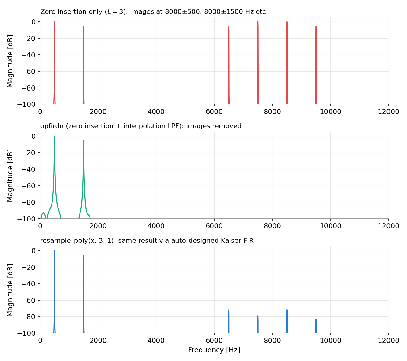
axes[0].set_title('Zero insertion only: images at 6.5/8.5/9.5 kHz etc.')
f1, S1 = spectrum_db(x_upfirdn, fs_up)
axes[1].plot(f1, S1, color='seagreen')
axes[1].set_title('upfirdn (zero insertion + LPF): images removed')
f2, S2 = spectrum_db(x_poly, fs_up)
axes[2].plot(f2, S2, color='navy')
axes[2].set_title('resample_poly(x, 3, 1): same result, auto-designed filter')
for ax in axes:
ax.set_ylabel('Magnitude [dB]')
ax.set_ylim(-100, 5)
ax.set_xlim(0, fs_up / 2)
ax.grid(True, alpha=0.3)
axes[2].set_xlabel('Frequency [Hz]')
plt.tight_layout()
plt.show()
With zero insertion alone, images appear at \(8000 \pm 500\) and \(8000 \pm 1500\) Hz (and beyond) at the 24 kHz rate; after the interpolation filter, only the original 500 / 1500 Hz components remain. For interpreting these spectra, see FFT-based spectral analysis and Window Functions and PSD .
Measured values: with zero insertion alone, the image of the 500 Hz component appears at 7500 Hz and 8500 Hz at the same amplitude as the original (0 dB). Filtering with upfirdn suppresses that band down to -102.3 dB, while resample_poly reaches -79.0 dB (see the figure below). The gap comes from the transition-band margin of the auto-designed Kaiser FIR — resample_poly picks a somewhat more conservative (faster but slightly looser) filter automatically.
Rational-Rate Resampling (L/M Conversion)
To convert the sampling rate by a rational factor \(L / M\) , connect upsampling (\(\uparrow L\) ) → low-pass filter → downsampling (\(\downarrow M\) ) in that order. Upsampling must come first — downsampling first would destroy information.
The single filter in the middle serves both as the interpolation filter (cutoff \(\pi / L\) ) and the anti-aliasing filter (cutoff \(\pi / M\) ):
\[H(e^{j\omega}) = \begin{cases} L & \left(|\omega| < \min\left(\dfrac{\pi}{L}, \dfrac{\pi}{M}\right)\right) \\ 0 & (\text{otherwise}) \end{cases} \tag{7}\]The classic example is CD-to-48 kHz conversion, where \(48000 / 44100 = 160 / 147\) .
import numpy as np
import matplotlib.pyplot as plt
from math import gcd
from scipy.signal import resample_poly

# --- 44.1 kHz -> 48 kHz conversion ---
fs_in, fs_out = 44100, 48000
g = gcd(fs_out, fs_in)
L, M = fs_out // g, fs_in // g
print(f"L/M = {L}/{M}")        # -> 160/147

# Convert a 1 kHz sine and check the accuracy
duration = 0.05
t_in = np.arange(0, duration, 1/fs_in)
x_in = np.sin(2*np.pi*1000*t_in)

x_out = resample_poly(x_in, L, M)
t_out = np.arange(len(x_out)) / fs_out

# Compare against the reference (the continuous sine sampled directly at 48 kHz)
x_ref = np.sin(2*np.pi*1000*t_out)
edge = 200                     # exclude filter transients at the edges
err = np.max(np.abs(x_out[edge:-edge] - x_ref[edge:-edge]))
print(f"Max error: {err:.2e}")  # -> around 6.68e-04 (set by the filter accuracy)

plt.figure(figsize=(10, 4))
plt.plot(t_in[:100]*1000, x_in[:100], 'o-', label='44.1 kHz input',
         markersize=4, alpha=0.7)
plt.plot(t_out[:109]*1000, x_out[:109], '.-', label='48 kHz output',
         markersize=4, alpha=0.7)
plt.xlabel('Time [ms]')
plt.ylabel('Amplitude')
plt.title('Rational resampling 44.1 kHz -> 48 kHz (L/M = 160/147)')
plt.legend()
plt.grid(True, alpha=0.3)
plt.tight_layout()
plt.show()
A single call resample_poly(x, 160, 147) performs high-quality rate conversion. Internally, the “upsample by 160, then downsample by 147” chain is implemented in a polyphase structure, costing roughly \(1/160\)
of a naive implementation. The next section explains how.
Polyphase Decomposition
The Waste in the Naive Implementation
Implementing the decimation of Eq. (3) naively means “run the full FIR filter at the input rate \(f_s\) , then keep only one output out of \(M\) ” — you compute and throw away \(M-1\) of every \(M\) outputs. For an FIR filter with \(N\) taps, that costs \(N f_s\) multiply-accumulate (MAC) operations per second.
Type-1 Polyphase Decomposition
Polyphase decomposition eliminates this waste. Split the filter \(H(z) = \sum_n h[n] z^{-n}\) into \(M\) subfilters (polyphase components) by taking every \(M\) -th coefficient:
\[H(z) = \sum_{p=0}^{M-1} z^{-p} E_p(z^M) \tag{8}\] \[E_p(z) = \sum_{n} h[nM + p] \, z^{-n} \qquad (p = 0, 1, \ldots, M-1) \tag{9}\]For example, with \(M = 3\) and \(h = [h_0, h_1, h_2, h_3, h_4, h_5]\) , the components are \(E_0 = [h_0, h_3]\) , \(E_1 = [h_1, h_4]\) , \(E_2 = [h_2, h_5]\) .
The Polyphase Decimator: Derivation
Let’s walk through the substitution of Eq. (8) into Eq. (3) explicitly. Eq. (3) reads
\[y[m] = \sum_{k} h[k] \, x[Mm - k] \tag{3'}\]Reparametrize the summation index \(k\) as \(k = nM + p\) (with \(p = 0, 1, \ldots, M-1\) and \(n\) ranging over all integers). As \(p\) runs from \(0\) to \(M-1\) and \(n\) runs over all integers, \(k = nM + p\) covers every integer exactly once — this is just the decomposition of the integers into residue classes modulo \(M\) . Under this substitution,
\[h[k] = h[nM + p] = e_p[n] \tag{9'}\]is exactly the definition in Eq. (9), and
\[x[Mm - k] = x\bigl(M m - nM - p\bigr) = x\bigl(M(m - n) - p\bigr) = x_p[m - n] \tag{10'}\]holds as well (the last equality is precisely the definition \(x_p[m] := x[Mm - p]\) ). Substituting both into Eq. (3’) gives the decimator output:
\[y[m] = \sum_{p=0}^{M-1} \sum_{n} e_p[n] \, x_p[m - n], \qquad x_p[m] = x[mM - p] \tag{10}\]In words: distribute the input into \(M\) low-rate streams \(x_p\) (a commutator), pass each stream through its short subfilter \(E_p\) , and sum. All filtering now runs at the output rate \(f_s / M\) , so the MAC count per second drops to
\[C_{\text{direct}} = N f_s \quad \longrightarrow \quad C_{\text{poly}} = M \cdot \frac{N}{M} \cdot \frac{f_s}{M} = \frac{N f_s}{M} \tag{11}\]a reduction by a factor of \(M\) . Interpolators can be polyphased in exactly the same way, saving a factor of \(L\) (multiplications by inserted zeros are skipped). Rational \(L/M\) converters benefit from both savings at once.
Python: Verifying a Polyphase Decimator
We implement Eq. (10) directly and confirm it matches both the naive “filter, then downsample” approach and scipy.signal.upfirdn.
import numpy as np
from scipy.signal import firwin, upfirdn

def polyphase_decimate(x, h, M):
    """Decimation in polyphase form (direct implementation of Eq. (10))."""
    N_out = len(x) // M
    y = np.zeros(N_out)
    for p in range(M):
        e_p = h[p::M]                        # subfilter E_p
        # low-rate input stream x_p[m] = x[mM - p]
        idx = np.arange(N_out) * M - p
        x_p = np.zeros(N_out)
        valid = idx >= 0
        x_p[valid] = x[idx[valid]]
        y += np.convolve(x_p, e_p)[:N_out]   # convolution at the low rate
    return y

# --- Verification ---
rng = np.random.default_rng(42)
fs, M = 48000, 4
x = rng.standard_normal(fs)                  # 1 second of white noise
h = firwin(128, 1/M)                         # FIR with cutoff pi/M

y_naive = np.convolve(x, h)[::M][:len(x)//M] # naive: full-rate filter -> downsample
y_poly = polyphase_decimate(x, h, M)
y_scipy = upfirdn(h, x, up=1, down=M)[:len(x)//M]

print("polyphase == naive :", np.allclose(y_poly, y_naive))   # True
print("polyphase == scipy :", np.allclose(y_poly, y_scipy))   # True

# --- Complexity comparison (theoretical) ---
N = len(h)
print(f"Direct form     : {N * fs / 1e6:.1f} M MAC/s")
print(f"Polyphase form  : {N * fs / M / 1e6:.1f} M MAC/s (1/{M})")
All three implementations produce identical outputs (polyphase == naive : True, polyphase == scipy : True). As a theoretical figure, for \(N=128\)
taps, \(f_s=48000\)
Hz, \(M=4\)
, the direct-form cost is “6.1 M MAC/s” versus the polyphase-form cost of “1.5 M MAC/s (1/4)”, matching the \(1/M\)
reduction of Eq. (11). scipy.signal.upfirdn and resample_poly implement this polyphase structure in C and never materialize the zero-stuffed intermediate signal.
Measuring the Real Speedup: A Gap Between Theory and Practice
The \(1/M\) reduction in Eq. (11) is a theoretical MAC-count figure. How much faster it actually runs in wall-clock time depends heavily on implementation overhead — Python function calls, array copies, and how efficiently NumPy vectorizes the loop. Let’s check this pitfall empirically.
import numpy as np
import timeit
from scipy.signal import firwin, upfirdn

rng = np.random.default_rng(42)
fs = 48000
x10 = rng.standard_normal(fs * 10)          # 10 seconds of audio-like data
N_taps = 2049                                # taps typical of a high-quality audio SRC filter

print("Timing scaling with M (fs=48kHz, 10s, N=2049 taps):")
for M_test in [2, 4, 8, 16, 32]:
    h_test = firwin(N_taps, 1 / M_test)

    def naive_f():
        return np.convolve(x10, h_test)[::M_test]

    def scipy_f():
        return upfirdn(h_test, x10, up=1, down=M_test)

    t_naive = timeit.timeit(naive_f, number=3) / 3
    t_scipy = timeit.timeit(scipy_f, number=3) / 3
    print(f"  M={M_test:2d}: naive={t_naive*1000:7.2f} ms, "
          f"upfirdn={t_scipy*1000:6.2f} ms, speedup={t_naive/t_scipy:.1f}x")
Actual output (Apple Silicon, Python 3.13 / NumPy 2.4 / SciPy 1.18):
M= 2: naive=171.73 ms, upfirdn=666.51 ms, speedup=0.3x
M= 4: naive=150.01 ms, upfirdn=314.85 ms, speedup=0.5x
M= 8: naive=170.04 ms, upfirdn=156.26 ms, speedup=1.1x
M=16: naive=149.46 ms, upfirdn= 78.21 ms, speedup=1.9x
M=32: naive=150.15 ms, upfirdn= 39.25 ms, speedup=3.8x
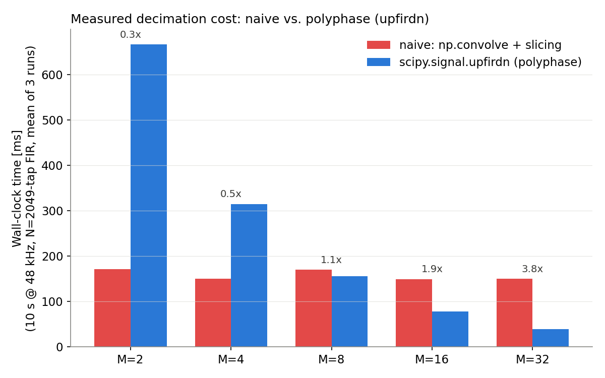
This is an important practical pitfall. np.convolve is a highly optimized direct convolution at the C level, so for small decimation factors (\(M=2, 4\)
), the overhead of upfirdn’s array bookkeeping and polyphase decomposition outweighs the theoretical computational savings, and the naive implementation is actually faster. As the figure and measurements show, the benefit of polyphase decomposition only becomes clearly visible in wall-clock time from roughly \(M \geq 8\)
onward. Don’t take the claim “polyphase decomposition is theoretically \(1/M\)
” at face value — benchmark it for your actual use case (the size of \(M\)
, the filter length, and the implementation you use). That said, in dedicated hardware (FPGA/ASIC) or SIMD-optimized C/C++ implementations, the raw operation count directly determines power consumption and circuit area, so the theoretical reduction retains its design value even for small \(M\)
.
Noble Identities
The correctness of the polyphase structure rests on the Noble identities — two equivalences for exchanging the order of filters and rate changers.
Downsampling side: downsampling by \(M\) followed by \(H(z)\) is equivalent to \(H(z^M)\) followed by downsampling by \(M\) :
\[\left(\downarrow M\right) \;\to\; H(z) \quad \equiv \quad H(z^M) \;\to\; \left(\downarrow M\right) \tag{12}\]Upsampling side: \(H(z)\) followed by zero insertion by \(L\) is equivalent to zero insertion followed by \(H(z^L)\) :
\[H(z) \;\to\; \left(\uparrow L\right) \quad \equiv \quad \left(\uparrow L\right) \;\to\; H(z^L) \tag{13}\]Here \(H(z^M)\) denotes the filter whose impulse response has \(M - 1\) zeros inserted between consecutive coefficients. Applying Eq. (12) to each term \(z^{-p} E_p(z^M)\) of the polyphase decomposition (Eq. 8) moves \(E_p(z^M)\) behind the downsampler — to the low-rate side — yielding the efficient structure of Eq. (10). The golden rule of multirate design, “always run filters on the low-rate side,” is guaranteed by these identities. The same rewriting is used to streamline multistage structures in wavelet filter banks and delta-sigma decimators.
Edge Cases and Pitfalls in Polyphase Implementations
Polyphase decomposition is powerful, but there are several pitfalls that are easy to overlook at implementation and design time.
Filter length \(N\)
not a multiple of \(M\)
: A naive implementation of Eq. (9), \(E_p(z) = \sum_n h[nM+p] z^{-n}\)
, gives subfilters whose lengths differ by up to one tap depending on \(p\)
(if \(N = qM + r\)
, then \(r\)
of the subfilters have \(q+1\)
taps and the remaining \(M-r\)
have \(q\)
taps). scipy.signal.upfirdn zero-pads internally to equalize this, but in a hand-rolled implementation, mishandling this remainder becomes a bug where only certain phases silently drop output samples. Deliberately choosing the tap count as \(N = kM\)
(integer \(k\)
) at design time avoids this altogether.
How linear phase is distributed: Even when the overall FIR filter \(h[n]\) is symmetric (linear phase), each individual polyphase component \(E_p(z)\) is generally not symmetric on its own. Linear phase is preserved as a symmetric relationship between branches (\(E_p\) and \(E_{M-1-p}\) are time-reversed versions of each other) — a single subfilter, viewed in isolation, can look asymmetric. The overall linear phase is only recovered once the branches are summed.
The special case of half-band filters: When \(M = 2\) (half-band), designing a filter whose passband and stopband edges are symmetric about half the Nyquist frequency makes every other coefficient (except the center tap) exactly zero. In that case, one of the two polyphase components (\(E_1\) ) degenerates into a plain integer delay (often just a single impulse), cutting the effective computation in half again. This is one reason \(\downarrow 2\) is so heavily used in two-channel QMF and wavelet filter banks.
The limits of rational-ratio approximation: The rational \(L/M\) conversion covered from Eq. (7) onward cannot, in principle, exactly realize an irrational target ratio (e.g., \(\sqrt{2}\) ). In practice, you pick \(L\) and \(M\) as a sufficiently close rational approximation (e.g., via continued fractions); larger \(L, M\) improve the approximation, but while the computational cost \(N f_s / M\) in Eq. (11) shrinks as \(M\) grows, the filter length \(N\) needed to hold a given stopband attenuation grows as the transition-band width \(\propto 1/\max(L,M)\) shrinks — so total computation does not necessarily improve monotonically. This trade-off matters for variable-ratio audio and communications rate conversion.
The gap between theoretical and measured cost: As the benchmark in the previous section showed, for small \(M\) (roughly \(M \leq 4\) ), NumPy/SciPy’s highly optimized direct convolution can outrun the polyphase implementation once overhead is accounted for. A theoretical reduction in operation count does not automatically translate into a shorter wall-clock time.
Choosing Between decimate, resample, and resample_poly
Here is a summary of SciPy’s three resampling functions.
| Function | Method | Supported ratios | Phase behavior | Edge behavior | Best suited for |
|---|---|---|---|---|---|
scipy.signal.decimate | LPF (IIR/FIR) + downsampling | Integer 1/M only | Zero phase with zero_phase=True | Filter transients | Integer-factor downsampling only |
scipy.signal.resample | FFT-based (truncate/extend in frequency) | Any (real-valued) | Zero phase | Assumes periodicity; ringing at aperiodic ends | Periodic, band-limited signals; offline analysis |
scipy.signal.resample_poly | Polyphase FIR (\(\uparrow L\) → LPF → \(\downarrow M\) ) | Rational \(L/M\) | Linear phase (group delay corrected) | Controllable via padtype | The default choice for real-world, streaming data |
scipy.signal.upfirdn | Polyphase FIR (bring your own filter) | Rational \(L/M\) | Depends on your filter | Zero padding | Rate conversion with custom filters, low-level control |
Practical guidelines:
- When in doubt, use
resample_poly: few artifacts even on aperiodic real data, and it handles rational ratios - Use
resampleonly when the signal is periodic or well band-limited; watch out for edge ringing decimateis a convenience function for integer-factor downsampling; apply it in stages for large \(M\)- If you need to control stopband attenuation or transition width yourself, design the FIR with
firwinetc. and pass it toupfirdn(see the Digital Filter Design Guide for the design flow)
Applications and Design Tips
| Application | Typical rate conversion | Key points |
|---|---|---|
| Audio sample-rate conversion | 44.1 kHz ↔ 48 kHz (160/147) | High-precision FIR (~ −100 dB stopband) in polyphase form |
| Delta-sigma ADC decimator | Several MHz → tens of kHz (large \(M\) ) | Cascade of CIC + multistage FIR, streamlined via Noble identities |
| Pulse shaping in comms | Interpolate to 4–8× symbol rate | Root-raised-cosine filter as a polyphase interpolator |
| Wavelet transform | \(\downarrow 2\) at every stage | Two-channel filter banks expressed as polyphase matrices |
| Preprocessing for spectral analysis | Downsample to the band of interest | Saves FFT size and frequency resolution |
Combining a bandpass filter with downsampling — bandpass decimation — is a standard technique for drastically reducing the computational load when analyzing narrowband signals.
Recent Research: Application to Neural Audio Processing
The challenge of “resampling while keeping computation low” that multirate processing addresses has recently become important in neural-network-based audio effect processing as well. Carson, Välimäki, Wright, and Bilbao’s paper “Resampling Filter Design for Multirate Neural Audio Effect Processing” (accepted for IEEE Transactions on Audio, Speech and Language Processing, 2025) proposes suppressing the aliasing that arises when running a neural audio effect model (e.g., a nonlinear guitar-amp simulator) at a sampling rate different from the one it was trained at — not by retraining the model, but by real-time resampling at the input and output stages. They show that “a two-stage design consisting of a half-band IIR filter cascaded with a Kaiser window FIR filter” matches or beats the previously proposed model-adjustment approach while using far fewer filtering operations per sample, with less than one millisecond of latency at typical audio rates. It’s a striking parallel that the “special efficiency of half-band filters” and “multistage decimation” ideas covered in this article are, in current practice, exactly what drives the computational savings in state-of-the-art neural audio processing (verified via WebFetch against the paper’s abstract; arXiv:2501.18470).
Summary
- Downsampling stretches the spectrum by \(M\) and superimposes copies, so an anti-aliasing filter with cutoff \(\pi/M\) is mandatory beforehand (= decimation)
- Upsampling creates spectral images through zero insertion, which are removed by an interpolation filter with gain \(L\) and cutoff \(\pi/L\)
- Rational \(L/M\) conversion is built as “\(\uparrow L\) → LPF → \(\downarrow M\) ”, with a single filter of cutoff \(\min(\pi/L, \pi/M)\) serving both roles
- Polyphase decomposition splits the filter into \(M\) subfilters running on the low-rate side, cutting the computation to \(1/M\) (or \(1/L\) for interpolators)
- The Noble identities justify exchanging filters and rate changers, underpinning the design principle “filters belong on the low-rate side”
- In SciPy,
resample_polyis the practical default; usedecimatefor integer-factor downsampling,resamplefor periodic signals, andupfirdnfor custom filters
Related Articles
- Nyquist-Shannon Sampling Theorem and Aliasing - The Nyquist frequency and aliasing theory that multirate processing builds on.
- Signal Reconstruction and Interpolation: Sinc, Linear, and Spline - A detailed treatment of sinc interpolation, the ideal interpolation filter.
- DTFT vs DFT vs FFT - The frequency-domain representations underlying the spectral analysis in this article (Eqs. 2 and 5).
- Discrete Signal Processing Fundamentals Roadmap - An integrated hub covering sampling, interpolation, DFT, and the Z-transform.
- FIR vs IIR Filters - Directly relevant to choosing the implementation of anti-aliasing/interpolation filters.
- Low-Pass Filter Design and Comparison - The basics of designing the LPF that precedes decimation.
- Digital Filter Design Guide - The design flow for custom filters to use with upfirdn.
- Fast Fourier Transform (FFT): Theory and Python Implementation - Used to verify the spectra of resampled signals.
- Window Functions and Power Spectral Density (PSD) - The theory behind the window functions used in the spectral plots here.
- Bandpass Filter Design: Theory and Python Implementation - The band-selection filter to combine with bandpass decimation.
- Time-Frequency Analysis Guide - Choosing analysis methods (STFT, wavelets, etc.) for the downsampled signal.
- MDCT (Modified DCT) and Filter Banks - Cosine-modulated filter banks and perfect reconstruction (TDAC), a natural extension of polyphase decomposition.
References
- Crochiere, R. E., & Rabiner, L. R. (1983). Multirate Digital Signal Processing. Prentice Hall.
- Vaidyanathan, P. P. (1993). Multirate Systems and Filter Banks. Prentice Hall.
- Oppenheim, A. V., & Schafer, R. W. (2009). Discrete-Time Signal Processing (3rd ed.). Prentice Hall.
- harris, f. j. (2004). Multirate Signal Processing for Communication Systems. Prentice Hall.
- Carson, A., Välimäki, V., Wright, A., & Bilbao, S. (2025). Resampling Filter Design for Multirate Neural Audio Effect Processing. IEEE Transactions on Audio, Speech and Language Processing. arXiv:2501.18470
- SciPy Signal Processing — decimate
- SciPy Signal Processing — resample_poly
- SciPy Signal Processing — upfirdn