Introduction
In Short-Time Fourier Transform (STFT): Theory and Python Implementation we covered the mathematical definition of the STFT and the time-frequency resolution trade-off (the uncertainty principle). This article is the practical sequel. Even with the theory in hand, the moment you actually plot a spectrogram you run into questions like:
- What value should
npersegbe? Is there a quantitative way to decide? - Should
noverlapbe 50% or 75%? What is the COLA condition, and when does it matter? - What is the difference between
scipy.signal.spectrogram,stft, andShortTimeFFT, and which one should I use? - When I modify a spectrogram and invert it, what happens to the phase?
This article answers these questions with design procedures, numerically verified code, and a legacy-to-new API mapping table. For choosing between analysis methods in the first place, see the time-frequency analysis selection guide .
How to Read a Spectrogram
The Three Axes and Display Range Design
A spectrogram is a 2D image with “horizontal axis = time (frame center), vertical axis = frequency, color = magnitude or power.” The upper edge of the frequency axis is the Nyquist frequency \(f_s / 2\) , a direct consequence of the sampling theorem . The first thing to design in practice is the color axis range:
\[S_{\text{dB}}[m, k] = 20 \log_{10}\left(|X[m, k]| + \epsilon\right) \tag{1}\]With a linear magnitude scale, the strongest component dominates the colormap and anything below about −20 dB (amplitude ratio 1/10) is essentially invisible. Use dB, set vmax to the signal’s peak level, and set vmin near the noise floor (rule of thumb: vmax − 60 to 80 dB) so that strong and weak components are visible simultaneously.
Example: Why the dB Scale Matters
We compare linear and dB displays on a signal containing a chirp, a steady tone, and a short burst, using the ShortTimeFFT class recommended since SciPy 1.12.
import numpy as np
import matplotlib.pyplot as plt
from scipy.signal import ShortTimeFFT
from scipy.signal.windows import hann

# --- Test signal: chirp + steady tone + short burst ---
fs = 8000
t = np.arange(0, 2.0, 1/fs)
rng = np.random.default_rng(0)
x = np.sin(2*np.pi*(100*t + 475*t**2))            # linear chirp 100 -> 2000 Hz
x += 0.5*np.sin(2*np.pi*3000*t)                   # steady 3000 Hz (-6 dB)
burst = (1.2 <= t) & (t < 1.25)
x[burst] += 1.5*np.sin(2*np.pi*1200*t[burst])     # 50 ms burst
x += 0.02*rng.standard_normal(len(t))             # noise floor

nperseg, hop = 512, 128                           # 75% overlap
SFT = ShortTimeFFT(hann(nperseg, sym=False), hop=hop, fs=fs,
                   scale_to='magnitude')
Sx = SFT.stft(x)                                  # complex matrix (257, n_frames)
S_db = 20*np.log10(np.abs(Sx) + 1e-10)

t_ax = SFT.t(len(x))                              # frame center times [s]
f_ax = SFT.f                                      # frequency bins [Hz]

fig, axes = plt.subplots(1, 2, figsize=(12, 4.5), sharey=True)
im0 = axes[0].pcolormesh(t_ax, f_ax, np.abs(Sx), shading='gouraud',
                         cmap='inferno')
axes[0].set_title('Linear magnitude: weak components invisible')
im1 = axes[1].pcolormesh(t_ax, f_ax, S_db, shading='gouraud',
                         cmap='inferno', vmin=-80, vmax=0)
axes[1].set_title('dB scale: chirp, tone, burst and noise floor visible')
for ax, im in zip(axes, [im0, im1]):
    ax.set_xlabel('Time [s]')
    fig.colorbar(im, ax=ax)
axes[0].set_ylabel('Frequency [Hz]')
plt.tight_layout()
plt.show()
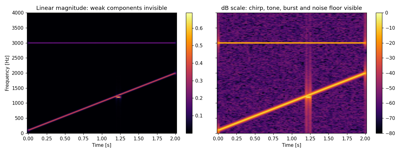
Rendering this confirms it directly: the linear-magnitude plot (left) shows almost nothing besides the chirp and the 3000 Hz tone. In the dB plot (right) you can identify everything at once: the diagonal chirp line, the horizontal 3000 Hz tone, the vertical burst at 1.2 s, and the uniform noise floor. Incidentally, the ridge of the chirp traces the instantaneous frequency at each time; for a mono-component signal the same trajectory can be extracted as a 1D signal via the Hilbert transform .
Logarithmic Frequency Axis
For music and audio, a log-frequency axis — where each octave (frequency ratio 2) occupies equal height — is often more natural. With pcolormesh this is a one-line change:
fig, ax = plt.subplots(figsize=(10, 4))
im = ax.pcolormesh(t_ax, f_ax, S_db, shading='gouraud',
                   cmap='inferno', vmin=-80, vmax=0)
ax.set_yscale('log')          # switch to log frequency axis
ax.set_ylim(50, fs/2)         # exclude DC (log axis cannot include 0)
ax.set_xlabel('Time [s]')
ax.set_ylabel('Frequency [Hz] (log)')
fig.colorbar(im, ax=ax, label='dB')
plt.tight_layout()
plt.show()
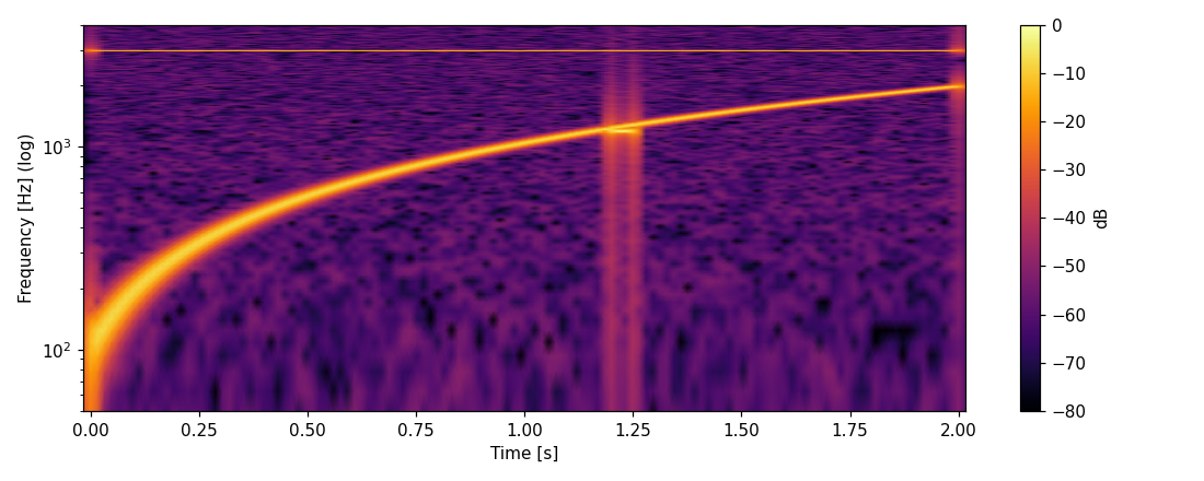
On the log axis, the linear chirp (whose frequency increases at a constant rate in Hz/s) appears to rise steeply at first and then flatten out, because equal frequency ratios occupy equal height on a log scale — the actual rate of change in Hz/s is constant throughout. Note that STFT bins remain linearly spaced, so the low-frequency region has only a few bins per octave. When low-frequency resolution is essential, switch to the wavelet transform (constant-Q analysis), whose window length scales with frequency.
Parameter Design in Practice
Window Length nperseg: Quantitative Resolution Design
The window length \(L\)
(nperseg) is the most important parameter. Two numbers drive the design.
(1) Bin spacing (the FFT frequency grid):
\[\Delta f_{\text{bin}} = \frac{f_s}{L} \tag{2}\](2) Effective frequency resolution — the minimum spacing at which two components can be separated. This is governed not by the bin spacing but by the mainlobe width of the window function:
\[\Delta f_{\text{res}} \approx k_w \cdot \frac{f_s}{L} \tag{3}\]where \(k_w\) is the window’s mainlobe width factor (derived in the window functions and PSD article ).
| Window | Mainlobe width \(k_w\) [bins] | Peak sidelobe | Practical role |
|---|---|---|---|
| Rectangular | 2 | −13 dB | Rarely used for spectrograms (heavy leakage) |
| Hann | 4 | −31 dB | The default choice |
| Hamming | 4 | −41 dB | When first-sidelobe suppression matters |
| Blackman | 6 | −58 dB | High dynamic range (hunting weak components) |
This yields a concrete design procedure:
- Decide the smallest frequency spacing \(\Delta f_{\min}\) you must separate (e.g., a semitone between musical notes, sideband spacing of a rotating machine)
- Pick a power of two with \(L \geq k_w \cdot f_s / \Delta f_{\min}\)
- Decide the fastest temporal event \(\Delta t_{\min}\) you must localize, and check that the window duration \(L / f_s\) does not exceed it
- If both cannot be met, either plot two spectrograms with different
nperseg, or switch to wavelets
For example, separating A4 (440 Hz) from A♯4 (466.16 Hz) — a 26 Hz gap — at \(f_s = 8000\)
Hz with a Hann window requires \(L \geq 4 \times 8000 / 26 \approx 1230\)
, i.e., nperseg=2048 or more. We verify this estimate numerically later.
noverlap: COLA and NOLA Conditions
noverlap determines the hop length \(H = L - \text{noverlap}\)
and plays two roles.
For display: the time-axis step of the spectrogram is \(H / f_s\) . If \(H\) is too large relative to \(L\) , events falling under the tapered edges of the window get underweighted. For Hann-family windows, 50–75% overlap (\(H = L/2\) to \(L/4\) ) is standard.
For reconstruction: inverting the STFT requires that the overlapping windows lose no information. Two conditions are used.
COLA (Constant OverLap-Add) — the window overlap sum is constant:
\[\sum_{m} w[n - mH] = C \quad (\forall n) \tag{4}\]NOLA (NonZero OverLap-Add) — the squared-window overlap sum never vanishes:
\[\sum_{m} w^2[n - mH] > 0 \quad (\forall n) \tag{5}\]NOLA is weaker than COLA and is the minimum requirement for the weighted overlap-add inverse STFT to be defined. SciPy provides checkers for both:
from scipy.signal import check_COLA, check_NOLA
from scipy.signal.windows import hann, hamming, blackman

nperseg = 512
windows = [('hann', hann(nperseg, sym=False)),
           ('hamming', hamming(nperseg, sym=False)),
           ('blackman', blackman(nperseg, sym=False))]
for name, w in windows:
    for ratio in (1/2, 2/3, 3/4):
        nov = int(nperseg * ratio)
        cola = check_COLA(w, nperseg, nov)
        nola = check_NOLA(w, nperseg, nov)
        print(f"{name:9s} overlap {ratio:.0%}: COLA={cola}, NOLA={nola}")
Output (verified with SciPy 1.18):
hann      overlap 50%: COLA=True, NOLA=True
hann      overlap 67%: COLA=False, NOLA=True
hann      overlap 75%: COLA=True, NOLA=True
hamming   overlap 50%: COLA=True, NOLA=True
hamming   overlap 67%: COLA=False, NOLA=True
hamming   overlap 75%: COLA=True, NOLA=True
blackman  overlap 50%: COLA=False, NOLA=True
blackman  overlap 67%: COLA=False, NOLA=True
blackman  overlap 75%: COLA=True, NOLA=True
Practical guidance:
- Display only: COLA is irrelevant; choose 50–75% to balance smoothness against compute cost
- Reconstruction: the periodic (
sym=False) Hann window with 50% or 75% overlap is the workhorse.ShortTimeFFT’s inverse works whenever NOLA holds, but COLA-satisfying combinations are numerically the most benign - Caution: even a seemingly innocent “2/3 overlap” can fail COLA. In any reconstruction pipeline, run
check_NOLAevery time you change parameters
Choosing the Window Function
For spectrograms, the general analysis in the window functions and PSD article applies directly. The short version: use Hann unless you have a reason not to; switch to Blackman-family windows when you need to see a weak component within ~40 dB of a strong neighbor. The rectangular window’s −13 dB sidelobes flood the noise floor and are almost never appropriate here.
nfft (mfft) and Zero Padding
Setting nfft (mfft in ShortTimeFFT) larger than nperseg zero-pads each frame before the FFT. The crucial point: zero padding interpolates the frequency axis but does not improve the effective resolution (mainlobe width). Resolution depends only on the actual data length \(L\)
inside the window. As explained in
DTFT, DFT, and FFT: sorting out the differences
, zero padding merely samples the DTFT on a finer grid.
In practice, mfft = 2 * nperseg is sometimes used to make peak frequencies easier to read off visually — but if you need to actually separate components, you must increase nperseg itself.
SciPy Old vs New API: From spectrogram / stft to ShortTimeFFT
SciPy 1.12 introduced the ShortTimeFFT class, and the older scipy.signal.stft / istft / spectrogram functions are now marked legacy in the official documentation (no removal is scheduled, but new code should use ShortTimeFFT).
Parameter Mapping Table
Legacy (stft / spectrogram) | ShortTimeFFT | Notes |
|---|---|---|
window='hann', nperseg=L | pass hann(L, sym=False) as 1st arg | The window is passed explicitly as an array |
noverlap | hop = nperseg - noverlap | Specified as a hop length, not an overlap |
nfft | mfft | FFT length after zero padding |
fs | fs | Same |
return values f, t, Zxx | SFT.f / SFT.t(len(x)) / stft(x) | Axes come from properties/methods |
boundary='zeros', padded=True | slices covering the signal by default | Controllable explicitly via p0, p1, k_offset |
scaling (stft uses spectrum) | scale_to='magnitude' | Amplitude-spectrum scaling |
spectrogram(mode='psd') | scale_to='psd' + spectrogram() | Watch the one-sided factor-of-2 (see below) |
istft(Zxx, ...) | SFT.istft(Sx, k1=len(x)) | Parameters automatically match the forward pass |
Verifying Numerical Equivalence
Let’s confirm the table numerically. Three subtleties: (1) legacy stft values match exactly with scale_to='magnitude' and phase_shift=None; (2) ShortTimeFFT also returns boundary slices at negative times, so the first slices must be aligned before comparison; (3) legacy spectrogram applies detrend='constant' by default and doubles all one-sided PSD bins except DC and Nyquist.
import numpy as np
from scipy.signal import stft, spectrogram, ShortTimeFFT
from scipy.signal.windows import hann

fs = 8000
t = np.arange(0, 2.0, 1/fs)
x = np.sin(2*np.pi*(100*t + 475*t**2)) + 0.5*np.sin(2*np.pi*3000*t)

nperseg, noverlap = 512, 384
hop = nperseg - noverlap
w = hann(nperseg, sym=False)

# (1) legacy stft
f_st, t_st, Zxx = stft(x, fs=fs, window=w, nperseg=nperseg,
                       noverlap=noverlap)

# (2) reproducing the same values with ShortTimeFFT
SFT = ShortTimeFFT(w, hop=hop, fs=fs, scale_to='magnitude',
                   phase_shift=None)
Sx = SFT.stft(x)
i0 = np.argmin(np.abs(SFT.t(len(x)) - t_st[0]))    # align first slices
print("stft == ShortTimeFFT:",
      np.allclose(Zxx, Sx[:, i0:i0 + Zxx.shape[1]]))          # True

# (3) legacy spectrogram (PSD mode) vs ShortTimeFFT
f_sp, t_sp, Sxx = spectrogram(x, fs=fs, window=w, nperseg=nperseg,
                              noverlap=noverlap, detrend=False)
SFT_psd = ShortTimeFFT(w, hop=hop, fs=fs, scale_to='psd')
S2 = SFT_psd.spectrogram(x)                        # = |STFT|^2
j0 = np.argmin(np.abs(SFT_psd.t(len(x)) - t_sp[0]))
S2 = S2[:, j0:j0 + Sxx.shape[1]].copy()
S2[1:-1] *= 2      # legacy one-sided PSD doubles non-DC/Nyquist bins
print("spectrogram == ShortTimeFFT:", np.allclose(Sxx, S2))   # True
Both comparisons print True (verified with SciPy 1.18). Bit-exact agreement of the complex STFT requires phase_shift=None; with ShortTimeFFT’s default phase_shift=0 the magnitudes agree but the phase convention differs — a trap to be aware of when migrating phase-sensitive code.
Which API to Use
- New code: use
ShortTimeFFT. Forward transform, inverse, spectrogram, and axis computation live on one object, so parameter mismatch bugs cannot occur - A quick one-off PSD plot: legacy
spectrogramremains perfectly serviceable (one line, Welch-convention PSD) - Migrating existing code: follow the pattern above (slice alignment, scaling, phase convention) and you can migrate while preserving numerical identity
Practice: Comparing Parameter Choices
Now let’s exercise the design procedure on a real task: “separate two tones 26 Hz apart (440 / 466.16 Hz) while also pinpointing 5 ms clicks.” From design equation (3), separating the tones with a Hann window needs \(L \geq 4 \times 8000 / 26 \approx 1230\) .
import numpy as np
import matplotlib.pyplot as plt
from scipy.signal import ShortTimeFFT
from scipy.signal.windows import hann

fs = 8000
t = np.arange(0, 1.5, 1/fs)
x = np.sin(2*np.pi*440*t) + np.sin(2*np.pi*466.16*t)   # A4 + A#4 (26 Hz apart)
for t0 in (0.4, 0.8, 1.2):                             # three 5 ms clicks
    m = (t >= t0) & (t < t0 + 0.005)
    x[m] += 3*np.sin(2*np.pi*2500*t[m])

fig, axes = plt.subplots(3, 1, figsize=(10, 10), sharex=True)
for ax, nperseg in zip(axes, [256, 1024, 4096]):
    hop = nperseg // 4                                 # 75% overlap
    SFT = ShortTimeFFT(hann(nperseg, sym=False), hop=hop, fs=fs,
                       scale_to='magnitude')
    S_db = 20*np.log10(np.abs(SFT.stft(x)) + 1e-10)
    im = ax.pcolormesh(SFT.t(len(x)), SFT.f, S_db, shading='gouraud',
                       cmap='inferno', vmin=-80, vmax=0)
    ax.set_ylim(0, 3000)
    ax.set_ylabel('Frequency [Hz]')
    ax.set_title(f'nperseg={nperseg}: bin spacing {fs/nperseg:.1f} Hz, '
                 f'Hann mainlobe {4*fs/nperseg:.0f} Hz, '
                 f'hop {hop/fs*1e3:.0f} ms')
    fig.colorbar(im, ax=ax, label='dB')
axes[-1].set_xlabel('Time [s]')
plt.tight_layout()
plt.show()
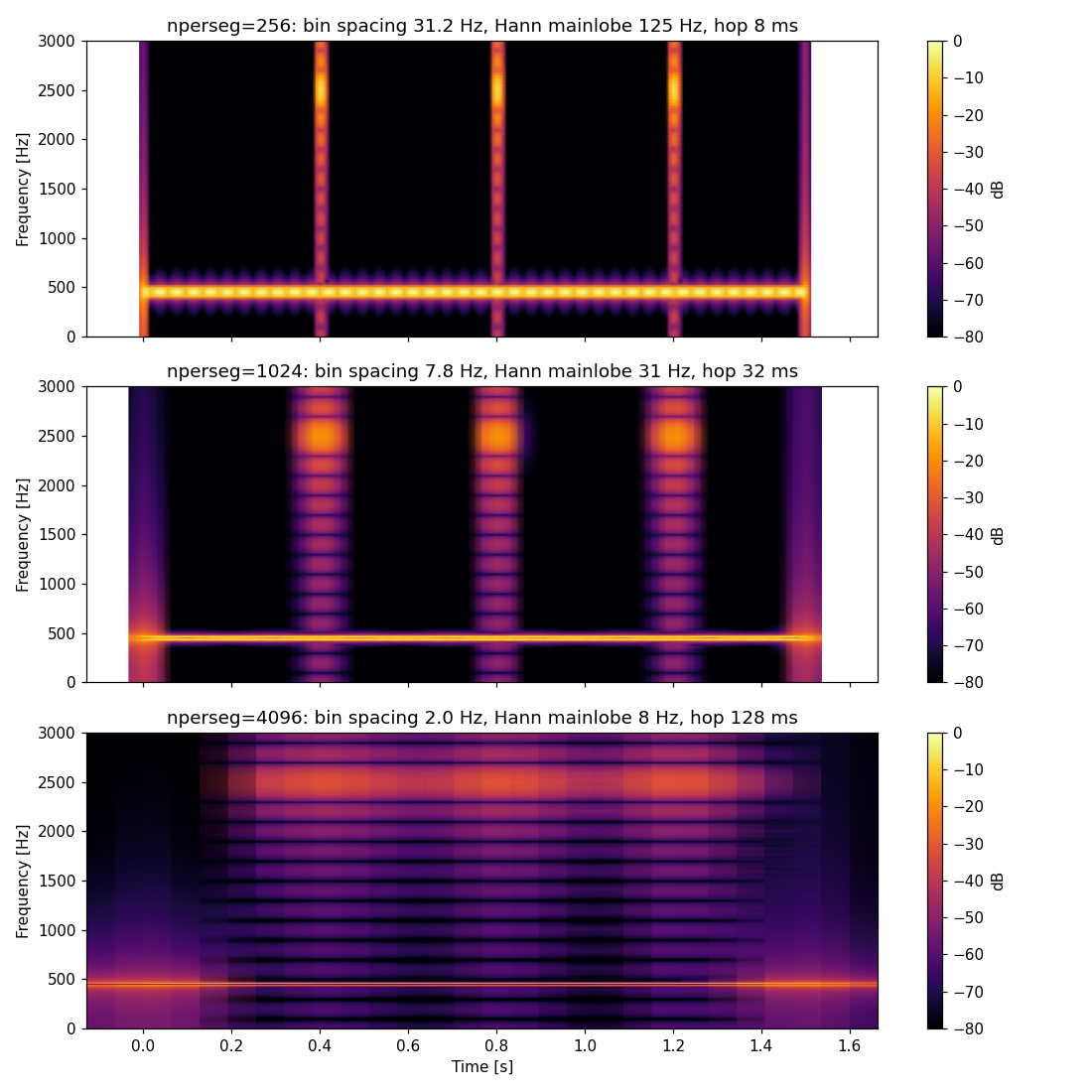
The apparent separability broadly matches the design equations:
nperseg | Mainlobe width | Two tones (26 Hz apart), full-view appearance | Clicks (5 ms) |
|---|---|---|---|
| 256 | 125 Hz | merged into a single band | sharp, clearly localized lines |
| 1024 | 31 Hz | looks like a single thick band (see below) | visible but thickened |
| 4096 | 8 Hz | clearly resolved into two lines | smeared across the 512 ms window |
But “separated in the full-view plot” and “actually separated at the bin level” are two different questions. Let’s take a 1D frequency cross-section at \(t = 0.6\)
s and overlay all three nperseg values:
idx = np.argmin(np.abs(SFT.t(len(x)) - 0.6))   # steady region, away from clicks
mask = (SFT.f > 395) & (SFT.f < 515)
plt.plot(SFT.f[mask], S_db[mask, idx])          # overlay one line per nperseg
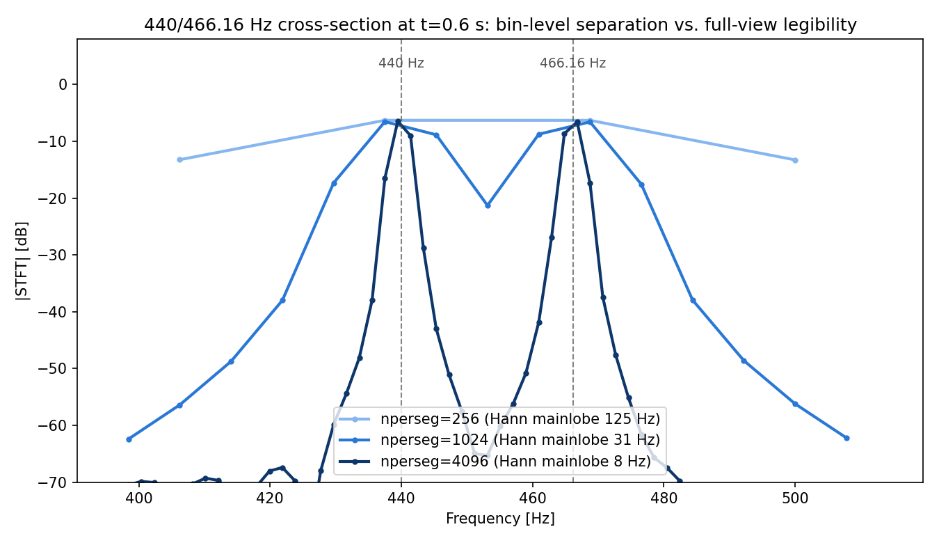
Measuring the “dip depth” (the average peak level minus the level at the midpoint, 453 Hz):
nperseg=256(mainlobe 125 Hz): dip depth 0.0 dB. The two peaks are fully merged into one hump — exactly as design equation (3) predicts.nperseg=1024(mainlobe 31 Hz): the mainlobe width (31 Hz) exceeds the 26 Hz spacing, so equation (3) alone would suggest “not separable.” But tracking the actual bin values reveals a dip depth of about 14.7 dB — the tones are separated at the bin level. The dip is simply too shallow to see in the full-view spectrogram (middle panel above), which is rendered over an 80 dB range.nperseg=4096(mainlobe 8 Hz): dip depth reaches about 58.8 dB, clearly visible as two lines even in the full-view plot.
Two lessons follow. (1) The mainlobe-width criterion in equation (3) is a conservative rule of thumb — a detectable dip can appear between bins even when the mainlobes nominally overlap. Real data has noise and unequal amplitudes, though, so a shallow dip is easily buried; for a robust separation you should still keep the margin equation (3) recommends (\(L \geq k_w f_s / \Delta f_{\min}\)
, i.e. nperseg=2048 or more here). (2) Whether a dip actually exists cannot always be judged from a fixed-vmin/vmax overview spectrogram alone — when in doubt, pull out a 1D frequency cross-section at a specific time and check directly.
Incidentally, when the two tones merge into a single bin (as at nperseg=256), tracking that bin’s amplitude over time reveals modulation from the beat between them (measured: the amplitude swings between about −13.2 and −2.2 dB with a period of roughly 1/26 s, i.e. 38 ms). This is a real instance of the uncertainty principle — two components unresolved on the frequency axis reappear as amplitude modulation on the time axis — but the swing is not large enough to read as a clear color variation in an 80 dB-range overview spectrogram. To visualize the beat, plot that bin’s amplitude directly as a 1D time series rather than relying on spectrogram color.
The takeaway: a single spectrogram cannot satisfy conflicting requirements. In practice, either (a) plot two spectrograms with different nperseg for the two purposes, or (b) switch to the
wavelet transform
when you need low-frequency resolution and transient localization simultaneously.
Inverse STFT and Signal Reconstruction
Reconstruction with ShortTimeFFT
ShortTimeFFT provides the inverse transform istft on the same object, and the invertible property tells you whether the NOLA condition (Eq. 5) holds:
SFT = ShortTimeFFT(hann(512, sym=False), hop=128, fs=fs,
                   scale_to='magnitude')
print("invertible:", SFT.invertible)               # True (NOLA satisfied)

Sx = SFT.stft(x)
x_rec = SFT.istft(Sx, k1=len(x))
print(f"max reconstruction error: {np.max(np.abs(x - x_rec)):.2e}")
# -> 6.66e-16 (perfect reconstruction at machine precision)
k1=len(x) specifies the original signal length. The legacy workflow of re-passing identical window / nperseg / noverlap values to istft is gone, which structurally eliminates a classic source of reconstruction bugs.
Filtering on the Spectrogram
Modifying STFT coefficients before inverting enables selective time-frequency processing. Here we remove everything above 2.5 kHz:
Sx_mod = Sx.copy()
Sx_mod[SFT.f > 2500, :] = 0        # zero all bins above 2.5 kHz
x_filt = SFT.istft(Sx_mod, k1=len(x))
Re-analyzing x_filt with the same SFT and comparing the 3000 Hz bin’s peak amplitude to the original shows the tone suppressed to about 0.84% of the original peak (verified with SciPy 1.18). The residual isn’t exactly zero because the inverse STFT’s overlap-add is a weighted reconstruction through the window function, so a little energy from the removed band leaks into neighboring frames and bins. By also masking along the time axis you can delete “this band at this moment only” — an operation impossible with a time-invariant
bandpass filter
. Speech denoising (spectral subtraction) and source-separation masking are direct extensions of this idea.
Phase Handling and the Griffin-Lim Algorithm
In the example above we modified only the magnitude and kept the original phase. There is a subtlety: the modified matrix \(\tilde{X}[m, k]\)
is generally not the STFT of any signal — the consistency between overlapping frames is broken. istft returns a least-squares-optimal signal for such an “inconsistent STFT,” so the stronger the modification, the larger the deviation from what you intended.
Furthermore, when only magnitudes are available — e.g., synthesizing audio from a mel spectrogram — the phase must be estimated from scratch. The classical method is the Griffin-Lim algorithm (GLA).
Formulation: given a target magnitude \(|X_{\text{target}}[m,k]|\) , GLA is an alternating projection between two constraint sets: (a) the consistency set \(\mathcal{C}\) (all matrices that are the valid STFT of some time-domain signal — projecting onto it means taking the ISTFT and then the STFT again), and (b) the magnitude set \(\mathcal{A}\) (all matrices whose entrywise magnitude equals \(|X_{\text{target}}|\) — projecting onto it means keeping the phase and replacing the magnitude). Each iteration is
\[ X_{i+1} = \mathcal{P}_{\mathcal{C}}\left(\mathcal{P}_{\mathcal{A}}(X_i)\right) \tag{6} \]Griffin & Lim (1984) proved that this iteration makes the consistency-error objective (\(\sum_{m,k} \bigl(|X_i[m,k]| - |X_{\text{target}}[m,k]|\bigr)^2\) -type quantity) monotonically non-increasing, converging to a critical point of that objective. That critical point is only a local optimum, however — there is no guarantee of reaching the global optimum or the true phase of whatever signal originally produced the target magnitude, and the result depends on the initial phase (commonly zero or random).
Fast Griffin-Lim (FGLA) (Perraudin et al., 2013) adds a Nesterov-style momentum term to accelerate convergence, but its convergence itself went unproven for roughly a decade. Nenov, Nguyen, Balazs, & Bot (2023) introduced a new inertial accelerated algorithm and, in the same work, gave the first convergence proof for FGLA.
Modern neural vocoders increasingly replace this iterative phase search entirely. Ai & Ling’s (2023) APNet, for example, predicts both the amplitude and phase spectra directly with two dedicated convolutional networks and reconstructs the waveform with a single inverse STFT — no GLA-style iteration required. Because it operates in parallel at the frame level, the authors report roughly 8x faster CPU inference than HiFi-GAN v1 at comparable quality. Where GLA searches iteratively for a phase consistent with a given magnitude, this line of work instead learns the joint amplitude-phase distribution directly from training data.
Toward Mel Spectrograms and Audio Preprocessing
In machine-learning pipelines for speech recognition and acoustic event detection, the standard input representation is the mel spectrogram — the linear-frequency spectrogram warped onto the perceptually motivated mel scale:
\[m = 2595 \log_{10}\left(1 + \frac{f}{700}\right) \tag{7}\]Implementation-wise it is just “STFT power spectrogram × mel filterbank (a stack of triangular filters),” so everything in this article about window length, hop, and window choice applies unchanged. In the audio field, librosa is the de facto standard library:
import librosa

# librosa: n_fft, hop_length and window have the same meaning as here
S_mel = librosa.feature.melspectrogram(
    y=x, sr=fs, n_fft=1024, hop_length=256,
    window='hann', n_mels=64
)
S_mel_db = librosa.power_to_db(S_mel, ref=np.max)
Taking the log of the mel spectrogram and applying a DCT yields MFCCs. This “spectrum of the log spectrum” structure is precisely cepstrum analysis ; MFCCs are the mel-scaled variant of the cepstrum.
Summary
- Display spectrograms in dB (range design:
vmax− 60 to 80 dB) and consider a log-frequency axis for music/audio - Design
npersegquantitatively so that the mainlobe width \(k_w f_s / L\) is smaller than the frequency spacing you must resolve (\(k_w = 4\) for Hann). Think in mainlobe width, not bin spacing \(f_s/L\) - Choose
noverlapat 50–75% for display; for reconstruction, satisfy NOLA (verify withcheck_NOLA/check_COLAwhenever parameters change) - Zero padding (
mfft>nperseg) is interpolation only — it never improves effective resolution ShortTimeFFTis the current SciPy API. It matches legacystftbit-exactly withscale_to='magnitude',phase_shift=None, and slice alignment; legacyspectrogram(PSD) additionally doubles interior one-sided bins- The inverse STFT via
SFT.istftachieves machine-precision reconstruction. Magnitude-modified STFTs are inconsistent, and phase-only-missing problems call for Griffin-Lim (alternating projection onto consistency and magnitude constraints, converging to a local optimum) or direct-prediction neural vocoders such as APNet - Mel spectrograms and MFCCs are direct applications of the STFT design covered here
Related Articles
- Short-Time Fourier Transform (STFT): Theory and Python Implementation - The theory prequel to this article: STFT definition, uncertainty principle, and basic implementation.
- How to Choose a Time-Frequency Analysis Method - A decision-flow guide comparing STFT, wavelets, and the Hilbert transform.
- Fast Fourier Transform (FFT): Theory and Python Implementation - The FFT algorithm applied to every STFT frame.
- Window Functions and Power Spectral Density (PSD) - The theory behind the mainlobe/sidelobe numbers used in this article’s window selection criteria.
- DTFT, DFT, and FFT: Sorting Out the Differences - Why zero padding is merely a finer sampling of the DTFT.
- Sampling Theorem and Aliasing - The theory fixing the upper edge (Nyquist frequency) of every spectrogram.
- Wavelet Transform: Theory and Python Implementation - Variable-length windows resolve what fixed-window STFT cannot.
- Hilbert Transform and Instantaneous Frequency - Extracts the chirp ridge seen in spectrograms as a 1D instantaneous-frequency signal.
- Cepstrum Analysis: Theory and Python Implementation - The “spectrum of a spectrum” analysis that leads from mel spectrograms to MFCCs.
- MDCT (Modified DCT) and Filter Banks - A frame-based time-frequency transform like the spectrogram, but with perfect reconstruction — the workhorse of audio compression.
References
- Griffin, D., & Lim, J. (1984). “Signal estimation from modified short-time Fourier transform.” IEEE Transactions on Acoustics, Speech, and Signal Processing, 32(2), 236-243.
- Nenov, R., Nguyen, D.-K., Balazs, P., & Bot, R. I. (2023). “Accelerated Griffin-Lim algorithm: A fast and provably converging numerical method for phase retrieval.” arXiv:2306.12504 .
- Ai, Y., & Ling, Z.-H. (2023). “APNet: An All-Frame-Level Neural Vocoder Incorporating Direct Prediction of Amplitude and Phase Spectra.” IEEE/ACM Transactions on Audio, Speech, and Language Processing.
- Smith, J. O. (2011). Spectral Audio Signal Processing. W3K Publishing.
- Oppenheim, A. V., & Schafer, R. W. (2009). Discrete-Time Signal Processing (3rd ed.). Prentice Hall.
- SciPy — ShortTimeFFT
- SciPy User Guide — Short-Time Fourier Transform (including the comparison with the legacy implementation)
- librosa — melspectrogram