Where This Article Fits
In the fundamentals article on Gaussian process regression we covered the GP definition, the closed-form posterior, and a from-scratch NumPy implementation. This is the hands-on sequel: we upgrade the “single RBF kernel with hand-picked hyperparameters” setup from the basics into something that survives contact with real data.
- Kernel design: choosing between RBF / Matérn / periodic / linear / WhiteKernel, and composing them with sums and products
- Hyperparameter optimization: log marginal likelihood maximization in practice, and escaping local optima with
n_restarts_optimizer - Using the predictive variance: reading confidence intervals and understanding why extrapolation is dangerous
- Scalability: the \(O(n^3)\) wall and Nyström / inducing-point approximations
All code in this article was executed and verified with scikit-learn 1.9 / NumPy 2.4.
Kernel Design in Practice
As the basics article showed, the kernel \(k(\mathbf{x}, \mathbf{x}')\) determines everything about a GP. Practical kernel design means enumerating the structures present in your data — smoothness, periodicity, trend, noise — and assembling the matching building blocks.
The Building Blocks
The main kernels in sklearn.gaussian_process.kernels:
| Kernel | Form (sketch) | Structure it encodes |
|---|---|---|
RBF(length_scale) | \(\exp(-r^2 / 2\ell^2)\) | Infinitely differentiable, smooth |
Matern(length_scale, nu) | Eq. (1) | Smoothness controlled by \(\nu\) |
ExpSineSquared(ls, p) | \(\exp\left(-\frac{2\sin^2(\pi r / p)}{\ell^2}\right)\) | Exact repetition with period \(p\) |
DotProduct(sigma_0) | \(\sigma_0^2 + \mathbf{x} \cdot \mathbf{x}'\) | Linear trend |
WhiteKernel(noise_level) | \(\sigma_n^2 \, \delta(\mathbf{x}, \mathbf{x}')\) | Observation noise |
ConstantKernel(constant) | \(\sigma_f^2\) | Amplitude scale (used in products) |
RationalQuadratic(ls, alpha) | \(\left(1 + \frac{r^2}{2\alpha\ell^2}\right)^{-\alpha}\) | Mixture of RBFs at many scales |
where \(r = \|\mathbf{x} - \mathbf{x}'\|\) .
The Matérn Kernel: How to Choose ν
The Matérn kernel exposes a smoothness parameter \(\nu\) :
\[ k_{\nu}(r) = \sigma_f^2 \frac{2^{1-\nu}}{\Gamma(\nu)} \left(\frac{\sqrt{2\nu}\, r}{\ell}\right)^{\nu} K_{\nu}\left(\frac{\sqrt{2\nu}\, r}{\ell}\right) \tag{1} \]The practical selection rules are simple:
- \(\nu = 1/2\) (exponential kernel): sample paths are continuous but nowhere differentiable — good for jagged, Brownian-like signals (financial data, rough physical measurements)
- \(\nu = 3/2\) : once differentiable; a sensible default for many real datasets
- \(\nu = 5/2\) : twice differentiable; the de facto standard as a Bayesian optimization surrogate — smooth but not unrealistically so
- \(\nu \to \infty\) : recovers the RBF kernel; infinitely differentiable and often too smooth for real data
Because \(\nu\) cannot be optimized by gradient descent (closed-form derivatives are only cheap at \(\nu = 1/2, 3/2, 5/2\) ), the standard workflow is to try discrete candidates and compare their log marginal likelihood (LML). Verified comparison code:
import numpy as np
from sklearn.gaussian_process import GaussianProcessRegressor
from sklearn.gaussian_process.kernels import Matern, WhiteKernel, ConstantKernel as C

rng = np.random.default_rng(42)
X = np.sort(rng.uniform(-4, 4, 40)).reshape(-1, 1)
y = np.sin(2 * X.ravel()) + 0.15 * np.abs(X.ravel()) * rng.standard_normal(40)

for nu in [0.5, 1.5, 2.5, np.inf]:
    kernel = C(1.0) * Matern(length_scale=1.0, nu=nu) + WhiteKernel(0.1)
    gpr = GaussianProcessRegressor(kernel=kernel, n_restarts_optimizer=5,
                                   random_state=0)
    gpr.fit(X, y)
    print(f"nu={nu}: LML={gpr.log_marginal_likelihood_value_:.3f}")
Output:
nu=0.5: LML=-24.069
nu=1.5: LML=-20.297
nu=2.5: LML=-19.103
nu=inf: LML=-17.822
On this dataset (a smooth sine with heteroscedastic noise) larger \(\nu\) wins; on jagged signals the ordering reverses. The takeaway: the LML lets you compare kernel structures themselves, not just tune parameters within one — this is the core of GP model selection.
Note that the RBF kernel also plays a central role in support vector machines , but the two frameworks use it very differently: SVMs use the kernel as a deterministic tool for margin maximization, while GPs use it as a covariance — i.e., a prior over functions.
Sums and Products: A Grammar for Kernels
Kernels are closed under two operations:
- Sum \(k_1 + k_2\) : superposition of independent components (\(f = f_1 + f_2\) with \(f_i \sim \mathcal{GP}(0, k_i)\) )
- Product \(k_1 \times k_2\) : modulation of one structure by another (e.g., periodic × RBF = a periodic pattern whose shape drifts slowly)
Common design patterns:
| Data structure | Kernel composition |
|---|---|
| Trend + seasonality + noise | DotProduct + ExpSineSquared + WhiteKernel |
| Slowly changing periodicity (temperature) | ExpSineSquared * RBF + WhiteKernel |
| Long-term trend + short-term variation | RBF(long ls) + RBF(short ls) + WhiteKernel |
| Input-dependent amplitude | DotProduct * RBF |
Sanity-Checking a Kernel with Prior Samples (sample_y)
The most reliable way to check whether a composed kernel encodes the structure you intended is to sample functions from the prior and look at them before fitting anything. Calling sample_y on an unfitted GaussianProcessRegressor draws from the prior:
X_plot = np.linspace(0, 10, 200).reshape(-1, 1)
kernel = C(0.1) * DotProduct(sigma_0=1.0) + ExpSineSquared(1.0, periodicity=3.0)
gp_prior = GaussianProcessRegressor(kernel=kernel)  # no fit = prior
samples = gp_prior.sample_y(X_plot, n_samples=3, random_state=0)
# samples.shape == (200, 3): do the draws look like "slope + oscillation"?
If the draws look like periodic waveforms riding on a trend, the design matches the intent; if not, revisit the components or their initial values. A few lines of code turn the abstract kernel into pictures — make this a habit every time you write a composite kernel.
Multidimensional Inputs and ARD (Automatic Relevance Determination)
For multidimensional inputs, give each dimension its own length scale with RBF(length_scale=[l1, l2, ...]) — this is ARD (Automatic Relevance Determination). During LML optimization, the length scales of irrelevant dimensions grow automatically, effectively removing those dimensions from the model. Verified run:
Xa = rng.uniform(-2, 2, (60, 2))
ya = np.sin(2 * Xa[:, 0]) + 0.05 * rng.standard_normal(60)  # x2 is irrelevant

kernel = C(1.0) * RBF(length_scale=[1.0, 1.0]) + WhiteKernel(0.1)
gpr = GaussianProcessRegressor(kernel=kernel, n_restarts_optimizer=10,
                               random_state=0)
gpr.fit(Xa, ya)
print(gpr.kernel_)
# 0.996**2 * RBF(length_scale=[0.925, 1e+05]) + WhiteKernel(noise_level=0.00233)
The relevant dimension \(x_1\) gets \(\ell_1 = 0.925\) while the irrelevant \(x_2\) is pushed to \(\ell_2 = 10^5\) (pinned at its upper bound) — feature selection falls out of marginal-likelihood maximization for free. After fitting, the inverse length scales serve as feature-importance scores.
Worked Example: Decomposing Trend + Periodicity + Noise
Let’s decompose synthetic data — a linear trend, a sine with period 2.5, and Gaussian noise — using the sum of the three matching components:
import numpy as np
from sklearn.gaussian_process import GaussianProcessRegressor
from sklearn.gaussian_process.kernels import (
    ExpSineSquared, DotProduct, WhiteKernel, ConstantKernel as C,
)

rng = np.random.default_rng(42)
X = np.linspace(0, 10, 80).reshape(-1, 1)
y = (0.5 * X.ravel()                                  # linear trend
     + 1.5 * np.sin(2 * np.pi * X.ravel() / 2.5)      # period 2.5
     + 0.3 * rng.standard_normal(80))                 # observation noise

kernel = (
    C(1.0) * DotProduct(sigma_0=1.0)                              # trend
    + C(1.0) * ExpSineSquared(length_scale=1.0, periodicity=3.0)  # seasonal
    + WhiteKernel(noise_level=0.1)                                # noise
)
gpr = GaussianProcessRegressor(kernel=kernel, n_restarts_optimizer=10,
                               normalize_y=True, random_state=0)
gpr.fit(X, y)
print(gpr.kernel_)   # kernel after hyperparameter optimization
print(gpr.log_marginal_likelihood_value_)
Output:
0.299**2 * DotProduct(sigma_0=1.04)
  + 4.33**2 * ExpSineSquared(length_scale=9.08, periodicity=2.49)
  + WhiteKernel(noise_level=0.0201)
LML: 26.260
Look at periodicity=2.49: starting from an initial guess of 3.0, the optimizer recovered the true period 2.5 from the data alone. The learned WhiteKernel value is an estimate of the noise variance, so a single fit simultaneously performs additive signal decomposition and noise estimation.
This additive trend + seasonal + noise viewpoint is dual to the state-space decomposition used by the Kalman filter (level + seasonal states). In fact, Matérn GPs admit an equivalent state-space representation that can be inferred in \(O(n)\) with the RTS smoother .
Hyperparameter Optimization
Log Marginal Likelihood: Formula and Intuition
The kernel hyperparameters \(\boldsymbol{\theta}\) (length scales, amplitudes, period, noise variance, …) are fitted by maximizing the log marginal likelihood (LML):
$$ \log p(\mathbf{y} \mid X, \boldsymbol{\theta}) = \underbrace{-\frac{1}{2}\mathbf{y}^T K_{\boldsymbol{\theta}}^{-1} \mathbf{y}}{\text{data fit}} \underbrace{- \frac{1}{2} \log |K{\boldsymbol{\theta}}|}_{\text{complexity penalty}}
- \frac{n}{2} \log 2\pi \tag{2} $$
with \(K_{\boldsymbol{\theta}} = K + \sigma_n^2 I\) . The first term rewards fitting the data; the second penalizes the “size” of the function class that \(\boldsymbol{\theta}\) can express, so Occam’s razor is built in — no cross-validation needed. Shrinking the length scale improves the data-fit term but inflates \(|K_{\boldsymbol{\theta}}|\) ; the optimum balances the two.
The gradient is available in closed form:
\[ \frac{\partial}{\partial \theta_j} \log p(\mathbf{y} \mid X, \boldsymbol{\theta}) = \frac{1}{2} \mathrm{tr}\!\left[ \left( \boldsymbol{\alpha}\boldsymbol{\alpha}^T - K_{\boldsymbol{\theta}}^{-1} \right) \frac{\partial K_{\boldsymbol{\theta}}}{\partial \theta_j} \right], \quad \boldsymbol{\alpha} = K_{\boldsymbol{\theta}}^{-1} \mathbf{y} \tag{3} \]scikit-learn feeds this analytic gradient to L-BFGS-B and optimizes in \(\log \boldsymbol{\theta}\) space, which is far better conditioned for scale parameters.
A Numeric Example: Data Fit vs. Complexity Penalty in a Tug-of-War
Let’s see how the two terms of Eq. (2) actually move, with concrete numbers. The full derivation of the multivariate-normal density lives in Eq. (8) of the fundamentals article ; here we measure how the two terms trade off as \(\ell\) varies, and why their sum peaks at an intermediate value.
For \(n=30\) points from \(y = \sin(1.5x) + \varepsilon\) (\(\varepsilon \sim \mathcal{N}(0, 0.15^2)\) ), fixing the noise variance at \(0.15^2\) and an RBF kernel, we evaluate both terms of Eq. (2) at three length scales: too short, too long, and the LML-maximizing optimum.
import numpy as np
from scipy.linalg import cho_factor, cho_solve
from sklearn.gaussian_process import GaussianProcessRegressor
from sklearn.gaussian_process.kernels import RBF, WhiteKernel, ConstantKernel as C

rng = np.random.default_rng(42)
n = 30
X = np.sort(rng.uniform(-5, 5, n)).reshape(-1, 1)
y = np.sin(1.5 * X.ravel()) + 0.15 * rng.standard_normal(n)
sigma_n2 = 0.15 ** 2

def rbf(X1, X2, ls):
    d2 = (X1 - X2.T) ** 2
    return np.exp(-d2 / (2 * ls ** 2))

def lml_terms(ls):
    K = rbf(X, X, ls) + sigma_n2 * np.eye(n)
    c, low = cho_factor(K, lower=True)
    alpha = cho_solve((c, low), y)
    data_fit = -0.5 * y @ alpha                         # term 1: data fit
    complexity = -0.5 * 2 * np.sum(np.log(np.diag(c)))  # term 2: complexity penalty
    const = -0.5 * n * np.log(2 * np.pi)
    return data_fit, complexity, const, data_fit + complexity + const

# optimal length scale found by LML maximization (same procedure as the next experiment)
kernel = C(1.0, "fixed") * RBF(length_scale=1.0) + WhiteKernel(sigma_n2, "fixed")
gpr = GaussianProcessRegressor(kernel=kernel, n_restarts_optimizer=10, random_state=0)
gpr.fit(X, y)
ls_opt = gpr.kernel_.k1.k2.length_scale

for ls, label in [(0.15, "too short"), (ls_opt, "ML-optimal"), (5.0, "too long")]:
    d, comp, const, tot = lml_terms(ls)
    print(f"l={ls:6.3f} [{label:10s}] data_fit={d:8.3f}  complexity={comp:7.3f}  LML={tot:8.3f}")
Output:
l= 0.150 [too short ] data_fit=  -6.076  complexity=  8.488  LML= -25.156
l= 1.075 [ML-optimal] data_fit=  -9.521  complexity= 35.808  LML=  -1.281
l= 5.000 [too long  ] data_fit=-332.097  complexity= 48.163  LML=-311.502
(The const term is a fixed \(-27.568\)
for \(n=30\)
and is omitted from the table but included in the LML total above.) The two terms move in opposite, monotonic directions as \(\ell\)
changes:
- Data-fit term \(-\frac12 \mathbf{y}^T K^{-1}\mathbf{y}\) : improves as \(\ell\) shrinks, since the fit can track the observations almost exactly (\(-6.076 \to -9.521 \to -332.097\) ; it worsens as \(\ell\) grows)
- Complexity penalty \(-\frac12 \log\lvert K\rvert\) : as \(\ell\) grows, rows of \(K\) become more correlated and its determinant \(\lvert K\rvert\) shrinks (fewer independent function shapes are representable, i.e. the model gets simpler), so this term itself increases (\(8.488 \to 35.808 \to 48.163\) )
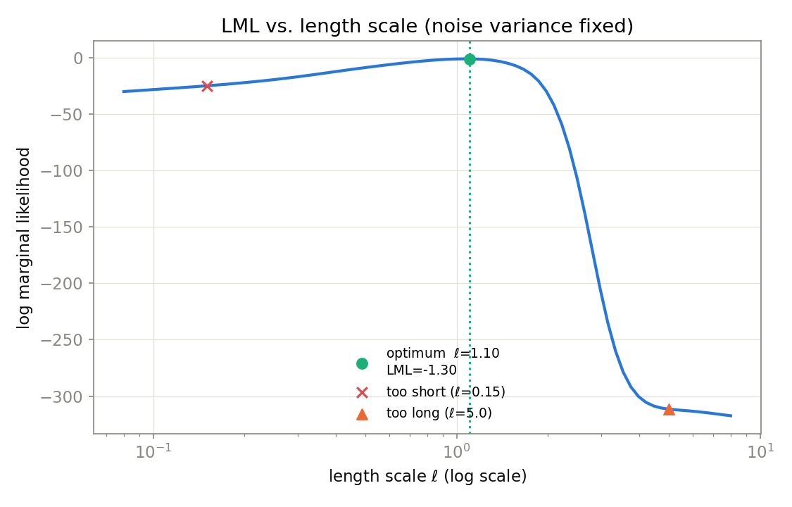
“Too short” gets a good data fit but barely benefits from the complexity term’s potential improvement, so the total loses badly (LML \(=-25.156\) ). “Too long” collapses the data fit so severely that no amount of complexity-side credit can compensate (LML \(=-311.502\) ). The ML-optimal \(\ell \approx 1.075\) sits exactly where the two balance, automatically selecting the least complexity needed without overreaching into the data — this is the concrete mechanism behind “Occam’s razor without cross-validation.”
Escaping Local Optima: n_restarts_optimizer
The LML is multimodal in \(\boldsymbol{\theta}\) . The classic failure mode has two competing explanations — “short length scale + tiny noise (memorize the data)” versus “long length scale + large noise (call the signal noise)” — each forming its own local optimum; periodic kernels additionally have optima at integer multiples and fractions of the true period.
The remedy is multi-start optimization via n_restarts_optimizer. Comparing on the composite kernel above:
for nr in [0, 10]:
    gpr = GaussianProcessRegressor(kernel=kernel, n_restarts_optimizer=nr,
                                   normalize_y=True, random_state=0)
    gpr.fit(X, y)
    print(f"n_restarts={nr}: LML={gpr.log_marginal_likelihood_value_:.3f}")
Output:
n_restarts= 0: LML=-85.099   # single run from the initial values -> stuck
n_restarts=10: LML= 26.260   # 10 restarts -> global optimum, period found
That is a 111-nat gap: without restarts the optimizer never discovers the periodic structure and settles on a completely different model. Practical guidance:
- Use
n_restarts_optimizer=10or more for composite kernels, especially ones containing a periodic component - Restart initial values are sampled log-uniformly from each hyperparameter’s
bounds, so tightening the bounds to physically plausible ranges directly improves search efficiency gpr.log_marginal_likelihood(theta)evaluates the LML at any \(\boldsymbol{\theta}\) — handy for convergence diagnostics and profile-likelihood plots
theta_opt = gpr.kernel_.theta.copy()          # optimized (log space)
print(gpr.log_marginal_likelihood(theta_opt))  # 26.260
theta_bad = theta_opt.copy()
theta_bad[-1] = np.log(1.0)                    # pin the noise variance at 1.0
print(gpr.log_marginal_likelihood(theta_bad))  # -84.535 -> noise estimation matters
Other Practical Switches
normalize_y=True: standardizes the targets to zero mean, unit variance. Since the GP prior mean is zero, this is near-mandatory for data with a large offsetalpha: jitter added to the diagonal (default \(10^{-10}\) ). Choose either learning the noise withWhiteKernelor fixing it viaalpha— using both duplicates the same role- Freezing hyperparameters: pass
length_scale_bounds="fixed"to exclude a parameter from optimization
Kernel-Selection Pitfalls and Numerical Caveats
Diagnosing Length-Scale Choice with LML and RMSE
Let’s actually fit GPR at three length scales — too short, too long, and the LML-maximizing optimum — and compare the resulting curves, LML, and held-out RMSE. We reuse the same dataset as the numeric example above: \(y = \sin(1.5x) + \varepsilon\) (\(n=30\) , \(\varepsilon \sim \mathcal{N}(0, 0.15^2)\) ).
from sklearn.metrics import mean_squared_error

X_test = np.linspace(-5, 5, 200).reshape(-1, 1)
y_test_true = np.sin(1.5 * X_test.ravel())

def eval_ls(ls, fitted_gpr=None):
    if fitted_gpr is None:  # fit fresh at a fixed length scale
        kernel = C(1.0, "fixed") * RBF(length_scale=ls, length_scale_bounds="fixed") + WhiteKernel(sigma_n2, "fixed")
        fitted_gpr = GaussianProcessRegressor(kernel=kernel)
        fitted_gpr.fit(X, y)
    mu, _ = fitted_gpr.predict(X_test, return_std=True)
    rmse = np.sqrt(mean_squared_error(y_test_true, mu))
    return fitted_gpr.log_marginal_likelihood_value_, rmse

# gpr is the model that already found ls_opt via n_restarts_optimizer=10 above
for ls, label, fitted in [(0.15, "too short", None), (ls_opt, "ML-optimal", gpr), (5.0, "too long", None)]:
    lml, rmse = eval_ls(ls, fitted)
    print(f"l={ls:6.3f} [{label:10s}] LML={lml:8.3f}  RMSE={rmse:.4f}")
Output:
| Length scale | LML | Held-out RMSE |
|---|---|---|
| \(\ell = 0.15\) (too short) | \(-25.156\) | \(0.3223\) |
| \(\ell = 1.075\) (optimal) | \(\bf-1.281\) | \(\bf0.1127\) |
| \(\ell = 5.0\) (too long) | \(-311.502\) | \(0.7046\) |
The length scale with the best LML also has the best RMSE — on this dataset, marginal-likelihood maximization is acting as a valid proxy for generalization performance (though this is not a general guarantee, as the recent-research section below discusses). Plotting all three fits makes the contrast obvious.
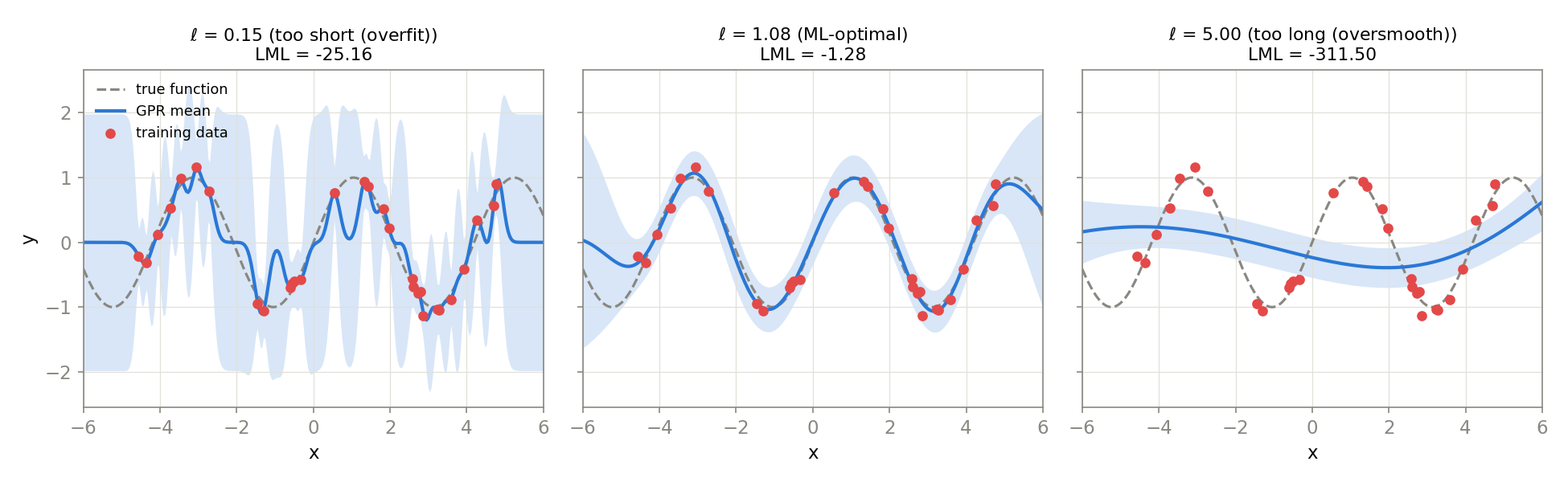
The leftmost panel (\(\ell=0.15\) ) essentially memorizes the observations and oscillates needlessly between them — overfitting. The rightmost panel (\(\ell=5.0\) ) flattens out the sine wave’s structure entirely — underfitting. The middle panel is what LML maximization picks automatically, and it tracks the true function most closely. Viewing this relationship as a continuous function of \(\ell\) shows the LML curve is unimodal and smooth, with the “too short” and “too long” candidates sitting far from its single peak.
Preventing Numerical Failure with Jitter
When observations sit close together, or the noise variance is set too small, the condition number of the kernel matrix \(K\)
degrades and the Cholesky factorization can fail outright. The
numerical-stability section
of the fundamentals article examines this in depth from the eigenvalue and runtime-speed angle, so here we focus on the practical scikit-learn workflow: controlling jitter through the alpha parameter and measuring its effect on predictions.
Feeding near-duplicate points (two pairs only \(10^{-7}\) apart, among 25 points) and near-noise-free data (\(\sigma \approx 10^{-4}\) ) causes the factorization to fail outright without jitter:
rng2 = np.random.default_rng(7)
n2 = 25
Xc = np.sort(rng2.uniform(-3, 3, n2)).reshape(-1, 1)
Xc[10, 0] = Xc[9, 0] + 1e-7   # near-duplicate points
Xc[20, 0] = Xc[19, 0] + 1e-7
yc = np.sin(2.0 * Xc.ravel()) + 1e-4 * rng2.standard_normal(n2)
Xc_test = np.array([[-2.5], [0.0], [2.5]])

for jit in [0.0, 1e-10, 1e-8, 1e-6, 1e-3]:
    kernel = C(1.0, "fixed") * RBF(length_scale=1.0, length_scale_bounds="fixed")  # no WhiteKernel
    gpr_j = GaussianProcessRegressor(kernel=kernel, alpha=jit)
    try:
        gpr_j.fit(Xc, yc)
        mu, std = gpr_j.predict(Xc_test, return_std=True)
        print(f"alpha={jit:.0e}: mu={np.round(mu,6)} std={np.round(std,6)}")
    except Exception as e:
        print(f"alpha={jit:.0e}: FAILED -> {type(e).__name__}")
Output:
alpha=0e+00: FAILED -> LinAlgError
alpha=1e-10: mu=[ 0.959363  0.000079 -0.958978] std=[6.0e-05 9.0e-06 2.7e-05]
alpha=1e-08: mu=[ 0.959162  0.000034 -0.959064] std=[4.41e-04 8.6e-05 1.96e-04]
alpha=1e-06: mu=[ 0.958913  0.000022 -0.958926] std=[0.002191 0.000735 0.001559]
alpha=1e-03: mu=[ 0.949461 -0.000019 -0.946445] std=[0.03122  0.020335 0.02718 ]
alpha=0 halts with scikit-learn’s own LinAlgError, telling you the kernel matrix “is not returning a positive definite matrix” and to gradually increase alpha — this is the numerical pitfall in its raw form. Adding jitter at the default-scale value \(10^{-10}\)
stabilizes the factorization, and the predictive mean shifts by at most \(4.5\times10^{-4}\)
compared to alpha=1e-6 (a relative error of roughly \(0.05\%\)
against a signal of scale \(\pm 1\)
). Push the jitter up to \(10^{-3}\)
, though, and the picture changes: the predictive standard deviation inflates nearly two orders of magnitude, from \(6\times10^{-5}\)
to \(0.031\)
, and the mean shifts by as much as \(0.0126\)
— at that point you’re effectively inflating the noise variance, not just stabilizing a factorization. The practical takeaway is simple: jitter should be the minimum needed to avoid failure. The default range of \(10^{-10}\)
to \(10^{-8}\)
typically prevents numerical breakdown without materially changing predictions, but pushing it up several orders of magnitude changes the model itself.
Using the Predictive Variance
Confidence Intervals
predict(X, return_std=True) returns the predictive mean \(\mu_*\)
and standard deviation \(\sigma_*\)
; the 95% confidence interval is \(\mu_* \pm 1.96\sigma_*\)
:
X_test = np.array([[5.0], [12.0], [20.0]])
mu, std = gpr.predict(X_test, return_std=True)
# x= 5.0 (interpolation):  mean= 2.503  std=0.240  95% CI=[ 2.033,  2.974]
# x=12.0 (extrapolation):  mean= 4.582  std=0.247  95% CI=[ 4.098,  5.065]
# x=20.0 (extrapolation):  mean=10.199  std=0.277  95% CI=[ 9.656, 10.742]
With return_cov=True you get the full covariance across test points, enabling posterior function sampling (sample_y) and joint confidence regions. The predictive variance also plugs straight into
time-series anomaly detection
: flag any observation outside \(\mu_* \pm 3\sigma_*\)
and you have a dynamic, model-based threshold for free.
The Danger of Extrapolation
In the numbers above, the prediction at \(x = 20\) — far outside the training range \([0, 10]\) — is 10.199 against a true value of 10.0. That only works because the kernel encodes global structure (linear + periodic). Solve the same kind of problem with a plain RBF kernel and the picture changes completely:
kernel_rbf = C(1.0) * RBF(length_scale=1.0) + WhiteKernel(noise_level=0.1)
# After fitting on the training range [0, 5]:
# x= 2.5 (interpolation): true= 2.188  mean= 2.102  std=0.083
# x= 6.0 (extrapolation): true= 2.249  mean= 1.096  std=1.285
# x=10.0 (extrapolation): true= 4.012  mean= 0.000  std=1.973
The RBF is a local kernel: correlation dies within a few length scales, so under extrapolation the mean reverts to the prior mean (zero) and the standard deviation returns to the prior amplitude \(\sigma_f \approx 1.97\) . Visualizing this over a wide range beyond the training window makes the smooth convergence to zero and the widening confidence band unmistakable (here, the RBF+WhiteKernel model with the LML-optimal \(\ell \approx 1.075\) found earlier, trained on \([-5, 5]\) and predicted out to \([-16, 16]\) ).
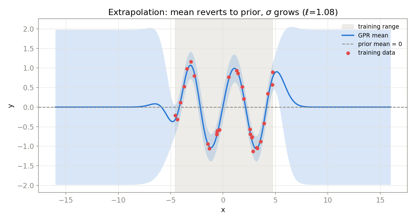
Near the center of the training range (well-interpolated) the standard deviation is about \(\sigma_* \approx 0.19\) , and past the edges of the training range (\(x=\pm 5\) ) it grows monotonically to nearly the prior standard deviation \(\sigma_f\sqrt{1+\sigma_n^2/\sigma_f^2} \approx 1.011\) by \(x=\pm 10\) and beyond, while the mean converges almost exactly to zero. Rather than a qualitative “uncertainty grows farther from the data,” GPR lets you estimate in advance exactly how far out this convergence happens and how large it gets — that predictability is the practical payoff. Two lessons:
- RBF/Matérn extrapolation returns an honest “I don’t know.” The exploding std is a feature, not a bug — this declared uncertainty is exactly what point-estimate models lack
- If you want structure to extend beyond the data, put that structure into the kernel explicitly (DotProduct for trends, ExpSineSquared for periodicity) — while recognizing this is a strong assumption that the structure continues out of range
Neural forecasters such as LSTMs and Transformers keep emitting confident-looking point forecasts under extrapolation, which is why GPR remains the first choice whenever calibrated prediction intervals are a hard requirement (safety constraints, inventory planning). For the bigger model-selection picture, see the time-series ML hub .
The Connection to Bayesian Optimization
The single most important application of GPR is as the surrogate model in Bayesian optimization. An expensive black-box function \(f\) is approximated by a GPR, and an acquisition function combines the predictive mean \(\mu_*\) (exploitation) with the predictive standard deviation \(\sigma_*\) (exploration) to pick the next evaluation point:
\[ \mathbf{x}_{\text{next}} = \arg\max_{\mathbf{x}} \; \alpha_{\text{EI}}(\mathbf{x}), \quad \alpha_{\text{EI}}(\mathbf{x}) = \mathbb{E}\left[\max(f_{\text{best}} - f(\mathbf{x}), 0)\right] \tag{4} \]Every practical topic in this article feeds directly into Bayesian optimization quality: Matérn \(\nu = 5/2\) is the de facto surrogate kernel, LML local optima degrade the surrogate (wasting expensive evaluations, hence restarts are mandatory), and the exploration term of the acquisition function is the predictive variance. For the derivation and implementation of EI / UCB / PI, see the Bayesian optimization fundamentals article .
The O(n³) Wall and Approximations
Exact GPR requires an \(O(n^3)\) Cholesky factorization of \(K_{\boldsymbol{\theta}} \in \mathbb{R}^{n \times n}\) and \(O(n^2)\) memory, hitting its limit around \(n \gtrsim 10^4\) — and since LML optimization repeats the factorization dozens of times, the practical ceiling is lower still. The main approximation families:
Nyström Approximation / SoR
Pick \(m \ll n\) inducing points \(Z = \{\mathbf{z}_1, \ldots, \mathbf{z}_m\}\) and low-rank-approximate the kernel matrix:
\[ K \approx \tilde{K} = K_{nm} K_{mm}^{-1} K_{mn} \tag{5} \]SoR (Subset of Regressors) replaces the GP with this \(\tilde{K}\) ; the Woodbury identity brings the cost down to \(O(nm^2)\) . In a verified run with \(n = 2000, m = 100\) , the SoR predictive mean matched the exact GP to within \(1.2 \times 10^{-7}\) — for smooth signals, 5% inducing points effectively reproduce the exact solution:
from scipy.linalg import cho_factor, cho_solve

idx = rng.choice(n, m, replace=False)
Z = X[idx]                              # inducing points (random subset)
K_mm = kernel(Z, Z) + 1e-8 * np.eye(m)
K_nm = kernel(X, Z)
A = K_mm * sn2 + K_nm.T @ K_nm          # reduce to m x m
c, low = cho_factor(A)
alpha = cho_solve((c, low), K_nm.T @ y)
mu = kernel(X_test, Z) @ alpha          # predictive mean in O(nm^2)
The catch: SoR underestimates the predictive variance (uncertainty collapses to zero away from the inducing points).
FITC / VFE / SVGP
- FITC: adds a diagonal correction to SoR, mitigating the variance collapse
- VFE (variational free energy): optimizes the inducing points themselves by maximizing a variational lower bound, so approximation quality is quantified as an LML bound
- SVGP: mini-batches VFE, scaling beyond \(n \sim 10^6\) ; available in GPyTorch / GPflow
Rule of thumb: exact GPR for \(n < 5{,}000\) ; VFE-family with \(m = 100\) –\(1000\) inducing points up to \(n < 10^5\) ; beyond that, SVGP or a switch to neural models.
Recent Research Trends
The three practical challenges covered here — LML maximization, escaping local optima with n_restarts_optimizer, and the \(O(n^3)\)
wall — are all active areas of improvement. Three representative developments since 2024:
Alternatives to LML that resist overfitting: This article treated LML maximization as “Occam’s razor without cross-validation,” but jointly optimizing many hyperparameters can let the LML itself overfit. Besginow, Hüwel, Pawellek, Beecks & Lange-Hegermann (2024) propose model-selection criteria based on the Laplace approximation, resolving an inconsistency in the naive Laplace approximation while matching nested-sampling-level accuracy at a fraction of the cost. Questioning the premise “higher LML at \(\theta\) = better model” directly reinforces the point made by this article’s numeric example — an overfit \(\ell\) can still improve the LML substantially.
A hybrid objective incorporating expected improvement: When the black-box function being modeled is expensive to evaluate, as in Bayesian optimization, LML maximization alone can leave the predictive variance poorly calibrated. Lualdi et al. (2024, Applied Soft Computing) propose a Hybrid Loss that augments the LML with a term derived from predictive uncertainty, improving the robustness of hyperparameter optimization for costly evaluation functions such as CFD/FEM simulations.
Faster LML optimization at scale: While this article addressed the \(O(n^3)\) wall mainly through inducing-point approximations, another line of work speeds up exact-GP LML optimization itself via iterative solvers (conjugate gradients). Lin, Padhy, Mlodozeniec, Antorán & Hernández-Lobato (2024, NeurIPS) combine warm-starting and early stopping in an iterative linear solver, letting the computation needed to evaluate the LML and its gradient carry over across multiple hyperparameter-update steps — bringing exact-GP hyperparameter optimization at scale closer to practical speeds.
Each of these addresses a different limitation of this article’s core prescription — “maximize the LML plus n_restarts_optimizer” — from a different angle: an objective that can overfit, calibration under expensive evaluation, and computational cost at scale.
Summary
| Topic | Practical takeaway |
|---|---|
| Kernel choice | Default to Matérn \(\nu \in \{3/2, 5/2\}\) ; compare structures via the LML |
| Composition | Sum = superposition, product = modulation; trend + periodic + WhiteKernel is the workhorse |
| Hyperparameters | Maximize the LML with n_restarts_optimizer>=10; tighten bounds to physical ranges |
| Predictive variance | 95% CI is \(\mu \pm 1.96\sigma\) ; variance blow-up under extrapolation is a feature — trust it |
| Scaling | Inducing-point approximations (SoR → VFE → SVGP) beyond \(n \gtrsim 10^4\) |
Describe your data’s structure in the language of kernels, then audit that description with the marginal likelihood — practical GPR is this loop, iterated.
Related Articles
- Gaussian Process Regression: Fundamentals and Python Implementation — the prerequisite: GP definition, posterior derivation, NumPy from-scratch implementation.
- Bayesian Optimization: Fundamentals and Python Implementation — the flagship application of GPR as a surrogate; EI / UCB / PI acquisition functions.
- Support Vector Machines (SVM): Kernel Methods and Nonlinear Classification — the deterministic branch of kernel methods, contrasted with kernels as covariances.
- SVM Kernel Design: Mercer’s Theorem, Gram-Matrix Positive Definiteness, and Random Fourier Features — the mathematical validity conditions (Mercer’s theorem, positive definiteness) behind every kernel used in this article; the theoretical grounding for kernel composition.
- Kalman Filter: Theory and Python Implementation — the state-space counterpart of additive decomposition; Matérn GPs run in O(n) via state space.
- Kalman Smoother (RTS): Forward-Backward Recursion and Python Implementation — full-interval smoothing, viewable as time-series-specialized GP regression.
- Time-Series Anomaly Detection: From Statistical Methods to Kalman Filter — using GPR prediction intervals as dynamic anomaly thresholds.
- LSTM for Time Series Forecasting: Theory and Python Implementation — the neural alternative for large data and long sequences.
- Time Series Forecasting with Transformers in PyTorch — the analogy between attention weights and kernel similarity.
- Machine Learning Hub for Time-Series Forecasting, Classification, and Anomaly Detection — the full model-selection map including GPR.
References
- Rasmussen, C. E., & Williams, C. K. I. (2006). Gaussian Processes for Machine Learning. MIT Press. (Especially Ch. 4 kernels, Ch. 5 model selection, Ch. 8 approximations.)
- Duvenaud, D. (2014). Automatic Model Construction with Gaussian Processes. PhD thesis, University of Cambridge. (The kernel-composition grammar.)
- Titsias, M. (2009). “Variational Learning of Inducing Variables in Sparse Gaussian Processes.” AISTATS 2009. (VFE)
- Hensman, J., Fusi, N., & Lawrence, N. D. (2013). “Gaussian Processes for Big Data.” UAI 2013. (SVGP)
- Besginow, A., Hüwel, J. D., Pawellek, T., Beecks, C., & Lange-Hegermann, M. (2024). “On the Laplace Approximation as Model Selection Criterion for Gaussian Processes.” arXiv:2403.09215.
- Lualdi, P., et al. (2024). “An Uncertainty-Based Objective Function for Hyperparameter Optimization in Gaussian Processes Applied to Expensive Black-Box Problems.” Applied Soft Computing. https://doi.org/10.1016/j.asoc.2024.111325
- Lin, J. A., Padhy, S., Mlodozeniec, B., Antorán, J., & Hernández-Lobato, J. M. (2024). “Improving Linear System Solvers for Hyperparameter Optimisation in Iterative Gaussian Processes.” NeurIPS 2024. arXiv:2405.18457.
- scikit-learn documentation: Gaussian Processes