Introduction: Filtering vs Smoothing
State estimation in state-space models comes in two flavors, depending on which observations you are allowed to use.
- Filtering: estimation using observations up to time \(k\) → \(p(x_k \mid y_{1:k})\) . This is a causal operation: the estimate can be updated as each observation arrives, making it suitable for online, real-time processing.
- Smoothing: estimation that also uses observations from the future → \(p(x_k \mid y_{1:T})\) with \(T > k\) . This is non-causal: exploiting future data always yields accuracy equal to or better than filtering, at the cost of latency.
Depending on “how far into the future you wait,” smoothers fall into three classes:
- Fixed-interval smoother: wait for the entire record \(y_{1:T}\) , then estimate \(\hat{x}_{k|T}\) for every \(k = 0, \ldots, T\) . The standard algorithm is the Rauch-Tung-Striebel (RTS) smoother . Fully offline.
- Fixed-lag smoother: always estimate the state \(N\) steps in the past, \(\hat{x}_{k-N|k}\) . Near-real-time processing with an acceptable delay of \(N\) steps.
- Fixed-point smoother: keep refining the estimate of one particular time \(j\) , \(\hat{x}_{j|k}\) , as new observations arrive. Used for initial-state or event-time estimation.
This article derives the recursions of all three smoothers, compares their complexity, latency, and use cases, and then benchmarks the Kalman filter, fixed-lag smoother, and RTS smoother with a from-scratch numpy implementation, measuring RMSE on the same simulated data.
For the underlying theory, see Kalman Filter: Theory and Python Implementation .
Comparison Table
Here is the summary up front. \(n\) is the state dimension, \(T\) the record length, \(N\) the lag.
| Aspect | Fixed-interval (RTS) | Fixed-lag | Fixed-point |
|---|---|---|---|
| Estimate | \(\hat{x}_{k\|T}\) for all \(k\) | \(\hat{x}_{k-N\|k}\) (always \(N\) steps behind) | \(\hat{x}_{j\|k}\) for one fixed \(j\) |
| Latency | full record (offline) | \(N\) steps (near real time) | none (incremental updates) |
| Cost / step | \(O(n^3)\) × forward + backward passes | \(O(N n^3)\) (windowed RTS) / \(O((Nn)^3)\) (augmented) | \(O(n^3)\) |
| Memory | \(O(T n^2)\) (all intermediate results) | \(O(N n^2)\) | \(O(n^2)\) |
| Accuracy | best (uses all observations) | approaches RTS as \(N \to \infty\) | approaches RTS at time \(j\) only |
| Typical use | batch analysis, trajectory reconstruction, EM | communications, speech enhancement, tracking | initial-state / event-time refinement |
Kalman Filter Review (Forward Pass)
All three smoothers consume the output of the Kalman filter forward pass. Define the linear Gaussian state-space model:
\[ x_k = F x_{k-1} + w_{k-1}, \quad w_{k-1} \sim \mathcal{N}(0, Q) \tag{1} \] \[ y_k = H x_k + v_k, \quad v_k \sim \mathcal{N}(0, R) \tag{2} \]Prediction Step
\[ \hat{x}_{k|k-1} = F \hat{x}_{k-1|k-1} \tag{3} \] \[ P_{k|k-1} = F P_{k-1|k-1} F^T + Q \tag{4} \]Update Step
\[ K_k = P_{k|k-1} H^T (H P_{k|k-1} H^T + R)^{-1} \tag{5} \] \[ \hat{x}_{k|k} = \hat{x}_{k|k-1} + K_k (y_k - H \hat{x}_{k|k-1}) \tag{6} \] \[ P_{k|k} = (I - K_k H) P_{k|k-1} \tag{7} \]For smoothing, we must store \(\hat{x}_{k|k}, P_{k|k}, \hat{x}_{k|k-1}, P_{k|k-1}\) at every step. For nonlinear systems, replacing equations \((3)\) –\((7)\) with the corresponding EKF or UKF steps yields nonlinear smoothers within the same framework.
Fixed-Interval Smoother (RTS)
Fixed-interval smoothing computes the posterior \(p(x_k \mid y_{1:T})\) for every time step using the whole record. The RTS smoother solves this with a backward recursion from \(T\) down to \(0\) .
Smoother gain:
\[ G_k = P_{k|k} F^T P_{k+1|k}^{-1} \tag{8} \]Smoothed state and covariance:
\[ \hat{x}_{k|T} = \hat{x}_{k|k} + G_k (\hat{x}_{k+1|T} - \hat{x}_{k+1|k}) \tag{9} \] \[ P_{k|T} = P_{k|k} + G_k (P_{k+1|T} - P_{k+1|k}) G_k^T \tag{10} \]The recursion starts from \(\hat{x}_{T|T}, P_{T|T}\) (the final forward-pass result) and runs for \(k = T-1, \ldots, 0\) . Since \(P_{k+1|T} \preceq P_{k+1|k}\) , we always have \(P_{k|T} \preceq P_{k|k}\) : smoothed uncertainty never exceeds filtered uncertainty. See the RTS smoother article for a full derivation.
Fixed-Lag Smoother
A fixed-lag smoother outputs the smoothed estimate \(\hat{x}_{k-N|k}\) — the state \(N\) steps in the past — every time a new observation \(y_k\) arrives. You keep streaming, yet each output has effectively “seen” \(N\) steps of the future.
Implementation 1: State Augmentation
Stack the last \(N+1\) states into an augmented state vector
\[ z_k = \begin{bmatrix} x_k^T & x_{k-1}^T & \cdots & x_{k-N}^T \end{bmatrix}^T \tag{11} \]and run a standard Kalman filter on the augmented system whose transition matrix shifts the blocks down by one (the Biswas–Mahalanabis fixed-lag smoother). Simple to implement, but the state dimension becomes \((N+1)n\) , so the cost grows as \(O((Nn)^3)\) .
Implementation 2: Windowed RTS (used below)
At each time \(k\) , run the RTS backward recursion (equations \((8)\) –\((9)\) ) only over the sliding window \([k-N, k]\) and output the estimate at the head of the window, \(\hat{x}_{k-N|k}\) . The per-step cost is \(O(N n^3)\) and only the last \(N\) forward-pass results need to be kept, so memory is \(O(N n^2)\) . Mathematically, this implementation treats the window’s endpoint \(k\) as if data had stopped there, and runs \(N\) steps of the RTS backward recursion from that artificial “end of the record.”
Implementations 1 (state augmentation) and 2 (windowed RTS) look completely different, yet they must compute the same quantity \(\hat{x}_{k-N|k}\) . We verify this agreement numerically in the “Python Implementation” section below.
The Lag-Length vs Accuracy Trade-off: Deriving the Variance-Gap Decay Law
We now derive, rather than just state, the “accuracy improves with \(N\) but saturates” behavior, using the RTS covariance recursion \((10)\) .
Fix a time \(j\) and let \(k\) be the window’s endpoint (recall that the windowed-RTS output’s covariance \(P_{j|k}\) is exactly equation \((10)\) evaluated with \(T=k\) ). Consider its gap from the covariance of the full-record RTS smoother, \(P_{j|T}\) :
\[ \delta_j^{(k)} := P_{j|k} - P_{j|T} \]Applying equation \((10)\) at time \(j\) for both horizons \(T=k\) and \(T\) (the true record length):
\[ P_{j|k} = P_{j|j} + G_j (P_{j+1|k} - P_{j+1|j}), \qquad P_{j|T} = P_{j|j} + G_j (P_{j+1|T} - P_{j+1|j}) \](\(G_j\) depends only on forward-pass quantities up to time \(j\) , so it is the same in both expressions.) Subtracting cancels the \(P_{j|j}\) and \(G_j P_{j+1|j}\) terms:
\[ \delta_j^{(k)} = G_j \left(P_{j+1|k} - P_{j+1|T}\right) G_j^T = G_j\, \delta_{j+1}^{(k)}\, G_j^T \tag{12} \]a clean backward recursion. Unrolling it for \(i = k-1, \ldots, j\) :
\[ \delta_j^{(k)} = \left(\prod_{i=j}^{k-1} G_i\right) \delta_k^{(k)} \left(\prod_{i=j}^{k-1} G_i\right)^{T} \]where \(\delta_k^{(k)} = P_{k|k} - P_{k|T}\) is simply the ordinary (zero-lag) filter-vs-RTS variance improvement. In steady state, \(G_i \to \bar{G}\) and \(\delta_k^{(k)} \to \bar\delta := \bar{P}_{k|k} - \bar{P}_{k|T}\) , so with \(N = k - j\) (the lag length; for a scalar system the transpose is just a second power):
\[ \delta_j^{(j+N)} \approx \bar{G}^{2N}\, \bar\delta \tag{13} \]The mean-level correction in equation \((9)\) decays like \(\bar{G}^N\) (a linear quantity, hit once by the gain \(G\) ), whereas the covariance (i.e., MSE) gap decays like \(\bar{G}^{2N}\) — twice as fast in the exponent — because it is hit twice, via the congruence transform \(G_j(\cdot)G_j^T\) . These are two independently derived facts, reflecting whether the estimator is linear or quadratic in the gain.
Ignoring bias, MSE equals variance, so \(\delta_k^{(k)} = \mathrm{MSE}_{\mathrm{KF}} - \mathrm{MSE}_{\mathrm{RTS}}\) , giving a prediction for the fixed-lag smoother’s MSE:
\[ \mathrm{MSE}_{\mathrm{lag}}(N) \approx \mathrm{MSE}_{\mathrm{RTS}} + \left(\mathrm{MSE}_{\mathrm{KF}} - \mathrm{MSE}_{\mathrm{RTS}}\right) \bar{G}^{2N} \tag{14} \]- Increasing \(N\) moves the accuracy toward RTS (which corresponds to \(N = \infty\) ), but the improvement saturates exponentially at rate \(\bar{G}^{2N}\)
- Latency and memory grow linearly in \(N\)
In practice, pick the smallest \(N\) for which \(\bar{G}^{2N}\) is negligible — typically a few multiples of the system time constant. We check how well equation \((14)\) ’s prediction matches the measured Monte Carlo RMSE later in this article.
Fixed-Point Smoother
The fixed-point smoother refines the estimate of one particular time \(j\) (e.g., the initial state or an event time), updating \(\hat{x}_{j|k}\) whenever a new observation \(y_k\) with \(k > j\) arrives. Rather than stating the update equations outright, we derive them from the RTS backward recursion.
Deriving the State Update: Telescoping the RTS Recursion
For \(j \le i \le k\) , define the “smoothing correction to the filter estimate” at time \(i\) as \(\Delta_i^{(k)} := \hat{x}_{i|k} - \hat{x}_{i|i}\) (so \(\Delta_k^{(k)} = 0\) ). Applying equation \((9)\) with \(T=k\) at time \(i\) :
\[ \Delta_i^{(k)} = \hat{x}_{i|k} - \hat{x}_{i|i} = G_i (\hat{x}_{i+1|k} - \hat{x}_{i+1|i}) \]Adding and subtracting \(\hat{x}_{i+1|i+1}\) :
\[ \Delta_i^{(k)} = G_i \left[ \big(\hat{x}_{i+1|k} - \hat{x}_{i+1|i+1}\big) + \big(\hat{x}_{i+1|i+1} - \hat{x}_{i+1|i}\big) \right] = G_i \left(\Delta_{i+1}^{(k)} + D_{i+1}\right) \tag{15} \]where \(D_{i+1} := \hat{x}_{i+1|i+1} - \hat{x}_{i+1|i} = K_{i+1} \nu_{i+1}\) (with \(\nu_{i+1} = y_{i+1} - H\hat{x}_{i+1|i}\) ) is a filter-only quantity that requires no smoothing at all. Unrolling equation \((15)\) for \(i = k-1, k-2, \ldots, j\) (starting from \(\Delta_k^{(k)}=0\) ):
\[ \Delta_j^{(k)} = \sum_{i=j+1}^{k} B_i D_i, \qquad B_i := \prod_{l=j}^{i-1} G_l \ \ (B_j = I) \tag{16} \]\(B_i\) itself satisfies the simple product recursion \(B_i = B_{i-1} G_{i-1}\) (\(B_j = I\) ). So \(\hat{x}_{j|k} = \hat{x}_{j|j} + \sum_{i=j+1}^{k} B_i K_i \nu_i\) , and taking the difference between horizon \(k-1\) and horizon \(k\) gives:
\[ \hat{x}_{j|k} = \hat{x}_{j|k-1} + B_k K_k \nu_k \tag{17} \]an \(O(n^3)\) update that runs every time a new observation arrives — this is the fixed-point smoother’s update equation.
Deriving the Covariance: Innovation Orthogonality
Let the error be \(e_j^{(k)} := x_j - \hat{x}_{j|k}\) . From equation \((16)\) , \(e_j^{(k)} = e_j^{(j)} - \sum_{i=j+1}^{k} B_i K_i \nu_i\) . Kalman filter innovations \(\nu_i\) are mutually uncorrelated (white noise), and for \(i > j\) , \(\nu_i\) is also uncorrelated with the estimation error \(e_j^{(j)}\) (innovation orthogonality, a standard Kalman filter property), so the covariance decomposes as a sum of independent terms:
\[ P_{j|k} = P_{j|j} - \sum_{i=j+1}^{k} B_i K_i S_i K_i^T B_i^T, \qquad S_i = H P_{i|i-1} H^T + R \]The one-step form of this recursion is \(P_{j|k} = P_{j|k-1} - B_k K_k S_k K_k^T B_k^T\) . Substituting the identity \(P_{k|k} - P_{k|k-1} = -K_k H P_{k|k-1} = -K_k S_k K_k^T\) (which follows from update equation \((7)\) and \(K_k = P_{k|k-1}H^T S_k^{-1}\) ):
\[ P_{j|k} = P_{j|k-1} + B_k (P_{k|k} - P_{k|k-1}) B_k^T \tag{18} \]which matches the equation stated at the top of this section. Equations \((17)\) –\((18)\) are \(O(n^3)\) per step with fixed \(O(n^2)\) memory, since only time \(j\) is tracked. Since \(B_k\) shrinks as \(k\) grows (the same mechanism as the decay law in equation \((13)\) ), the updates fade out and \(\hat{x}_{j|k}\) converges to the fixed-interval estimate \(\hat{x}_{j|T}\) .
The fixed-point smoother is used for high-accuracy estimation of the initial state \(x_0\) (as a preprocessing step for parameter estimation) and for refining event times, but implementing this recursion directly — without embedding it into an augmented state — is numerically delicate; a new Cholesky-based stabilization was proposed as recently as 2024 (see “Recent Research” below).
Python Implementation: RMSE Benchmark on a Random Walk
We compare the Kalman filter, fixed-lag smoother, and RTS smoother on the simplest possible system: a 1-D random walk observed in noise.
Model Definition
\[ x_k = x_{k-1} + w_{k-1}, \quad y_k = x_k + v_k, \quad w \sim \mathcal{N}(0, 0.05), \; v \sim \mathcal{N}(0, 1) \tag{19} \]import numpy as np
# ---- State-space model: random walk + observation noise ----
T = 300 # number of time steps
F = np.array([[1.0]]) # state transition (random walk)
H = np.array([[1.0]]) # observation matrix
Q = np.array([[0.05]]) # process noise variance
R = np.array([[1.0]]) # observation noise variance
n, m = 1, 1
x0 = np.array([0.0])
P0 = np.diag([1.0])
Kalman Filter (Forward Pass)
def kalman_filter(y_obs, F, H, Q, R, x0, P0):
    """Kalman filter forward pass (stores all intermediates for smoothing)"""
    T = len(y_obs)
    n = len(x0)
    x_filt = np.zeros((T + 1, n))       # x_{k|k}
    P_filt = np.zeros((T + 1, n, n))    # P_{k|k}
    x_pred = np.zeros((T, n))           # x_{k|k-1}
    P_pred = np.zeros((T, n, n))        # P_{k|k-1}
    x_filt[0], P_filt[0] = x0, P0
    for k in range(T):
        # Prediction (eqs. 3, 4)
        x_pred[k] = F @ x_filt[k]
        P_pred[k] = F @ P_filt[k] @ F.T + Q
        # Update (eqs. 5, 6, 7)
        S = H @ P_pred[k] @ H.T + R
        K = P_pred[k] @ H.T @ np.linalg.inv(S)
        x_filt[k + 1] = x_pred[k] + K @ (y_obs[k] - H @ x_pred[k])
        P_filt[k + 1] = (np.eye(n) - K @ H) @ P_pred[k]
    return x_filt, P_filt, x_pred, P_pred
RTS Smoother (Backward Pass)
def rts_smoother(x_filt, P_filt, x_pred, P_pred, F):
    """RTS (fixed-interval) smoother backward pass"""
    T = len(x_pred)
    n = x_filt.shape[1]
    x_smooth = np.zeros((T + 1, n))
    P_smooth = np.zeros((T + 1, n, n))
    x_smooth[T], P_smooth[T] = x_filt[T], P_filt[T]
    for k in range(T - 1, -1, -1):
        G = P_filt[k] @ F.T @ np.linalg.inv(P_pred[k])  # eq. 8
        x_smooth[k] = x_filt[k] + G @ (x_smooth[k + 1] - x_pred[k])  # eq. 9
        P_smooth[k] = P_filt[k] + G @ (P_smooth[k + 1] - P_pred[k]) @ G.T  # eq. 10
    return x_smooth, P_smooth
Fixed-Lag Smoother (Windowed RTS)
def fixed_lag_smoother(y_obs, F, H, Q, R, x0, P0, N):
    """Fixed-lag smoother: at each time k, run the backward recursion over
    the last N steps only and output x_{k-N|k} (windowed-RTS implementation)"""
    T = len(y_obs)
    n = len(x0)
    x_filt, P_filt, x_pred, P_pred = kalman_filter(y_obs, F, H, Q, R, x0, P0)
    x_lag = np.zeros((T + 1, n))
    x_lag[0] = x0
    for k in range(1, T + 1):
        j0 = max(0, k - N)  # time index k-N to output
        xs = x_filt[k].copy()
        for j in range(k - 1, j0 - 1, -1):  # backward recursion over [j0, k]
            G = P_filt[j] @ F.T @ np.linalg.inv(P_pred[j])
            xs = x_filt[j] + G @ (xs - x_pred[j])
        x_lag[j0] = xs
    # The last N points have no future observations yet; fill them with
    # the backward recursion of the final window
    xs = x_filt[T].copy()
    x_lag[T] = xs
    for j in range(T - 1, max(0, T - N) - 1, -1):
        G = P_filt[j] @ F.T @ np.linalg.inv(P_pred[j])
        xs = x_filt[j] + G @ (xs - x_pred[j])
        x_lag[j] = xs
    return x_lag
Numerical Agreement of the Two Fixed-Lag Implementations
We now verify the claim from the theory section — that implementation 1 (state augmentation) and implementation 2 (windowed RTS) must compute the same quantity — by actually implementing both.
def fixed_lag_augmented(y_obs, F, H, Q, R, x0, P0, N):
    """Biswas-Mahalanabis style: run a standard Kalman filter on the augmented
    state z_k = [x_k; x_{k-1}; ...; x_{k-N}] and read off the last block (= x_{k-N|k})"""
    n = len(x0)
    T = len(y_obs)
    B = N + 1
    A = np.zeros((B * n, B * n))
    A[0:n, 0:n] = F                                    # only the top block obeys the transition
    for i in range(1, B):
        A[i * n:(i + 1) * n, (i - 1) * n:i * n] = np.eye(n)  # the rest just shift (copy the previous block)
    Q_aug = np.zeros((B * n, B * n))
    Q_aug[0:n, 0:n] = Q                                 # process noise only enters the top block
    H_aug = np.zeros((H.shape[0], B * n))
    H_aug[:, 0:n] = H                                   # only the top block (x_k) is observed
    z0 = np.tile(x0, B)
    P0_aug = np.tile(P0, (B, B))                        # at t=0 every block is fully correlated with x0

    z_filt = np.zeros((T + 1, B * n))
    Pz_filt = np.zeros((T + 1, B * n, B * n))
    z_filt[0], Pz_filt[0] = z0, P0_aug
    for k in range(T):
        z_pred = A @ z_filt[k]
        P_pred_aug = A @ Pz_filt[k] @ A.T + Q_aug
        S = H_aug @ P_pred_aug @ H_aug.T + R
        K = P_pred_aug @ H_aug.T @ np.linalg.inv(S)
        z_filt[k + 1] = z_pred + K @ (y_obs[k] - H_aug @ z_pred)
        Pz_filt[k + 1] = (np.eye(B * n) - K @ H_aug) @ P_pred_aug

    x_lag = np.zeros((T + 1, n))
    for k in range(T + 1):
        j0 = max(0, k - N)
        depth = k - j0                                  # block holding x_{j0} at filtering time k
        x_lag[j0] = z_filt[k, depth * n:(depth + 1) * n]
    for i in range(B):                                  # the last N points: read directly off the final filter state
        x_lag[T - i] = z_filt[T, i * n:(i + 1) * n]
    return x_lag


rng_eq = np.random.default_rng(99)
x_true_eq = np.zeros((T + 1, n))
y_obs_eq = np.zeros((T, m))
for k in range(T):
    x_true_eq[k + 1] = F @ x_true_eq[k] + rng_eq.multivariate_normal(np.zeros(n), Q)
    y_obs_eq[k] = H @ x_true_eq[k + 1] + rng_eq.multivariate_normal(np.zeros(m), R)

for N in [1, 2, 3, 5]:
    x_lag_win = fixed_lag_smoother(y_obs_eq, F, H, Q, R, x0, P0, N)
    x_lag_aug = fixed_lag_augmented(y_obs_eq, F, H, Q, R, x0, P0, N)
    # skip the startup transient, where the augmented state's initial padding
    # (every block filled with x0) still lingers
    diff = np.abs(x_lag_win[N + 5:, 0] - x_lag_aug[N + 5:, 0])
    print(f"N={N}: max |windowed-RTS - augmented| = {diff.max():.3e}, mean = {diff.mean():.3e}")
Output:
N=1: max |windowed-RTS - augmented| = 4.441e-16, mean = 3.536e-17
N=2: max |windowed-RTS - augmented| = 4.441e-16, mean = 5.581e-17
N=3: max |windowed-RTS - augmented| = 4.441e-16, mean = 8.235e-17
N=5: max |windowed-RTS - augmented| = 8.882e-16, mean = 9.623e-17
The maximum difference is on the order of \(10^{-15}\) — within double-precision floating-point rounding error, i.e., an exact match. Two derivations with completely different formulations (reducing to a standard Kalman filter via state augmentation, versus truncating the RTS backward recursion to a window) provably yield the same estimator, and this is confirmed numerically.
Monte Carlo Evaluation (50 Runs)
A single realization can shuffle the ranking due to sampling noise, so we generate 50 sequences with numpy.random.default_rng and compare the average RMSE.
def rmse(a, b):
    return np.sqrt(np.mean((a - b) ** 2))

n_trials = 50
lags = [1, 2, 3, 5, 10, 20]
rmse_kf_list, rmse_rts_list = [], []
rmse_lag_lists = {N: [] for N in lags}

rng = np.random.default_rng(42)
for trial in range(n_trials):
    # Generate the true states and observations
    x_true = np.zeros((T + 1, n))
    y_obs = np.zeros((T, m))
    for k in range(T):
        x_true[k + 1] = F @ x_true[k] + rng.multivariate_normal(np.zeros(n), Q)
        y_obs[k] = H @ x_true[k + 1] + rng.multivariate_normal(np.zeros(m), R)

    x_filt, P_filt, x_pred, P_pred = kalman_filter(y_obs, F, H, Q, R, x0, P0)
    x_rts, P_rts = rts_smoother(x_filt, P_filt, x_pred, P_pred, F)

    rmse_kf_list.append(rmse(x_true[1:, 0], x_filt[1:, 0]))
    rmse_rts_list.append(rmse(x_true[1:, 0], x_rts[1:, 0]))
    for N in lags:
        x_lag = fixed_lag_smoother(y_obs, F, H, Q, R, x0, P0, N)
        rmse_lag_lists[N].append(rmse(x_true[1:, 0], x_lag[1:, 0]))

rmse_kf = np.mean(rmse_kf_list)
rmse_rts = np.mean(rmse_rts_list)
print(f"KF  filter RMSE : {rmse_kf:.4f}")
for N in lags:
    r = np.mean(rmse_lag_lists[N])
    print(f"Fixed-lag N={N:2d}   : {r:.4f}  ({(1 - r / rmse_kf) * 100:.1f}% improvement)")
print(f"RTS smoother    : {rmse_rts:.4f}  ({(1 - rmse_rts / rmse_kf) * 100:.1f}% improvement)")
Results
KF  filter RMSE : 0.4519
Fixed-lag N= 1   : 0.4145  (8.3% improvement)
Fixed-lag N= 2   : 0.3890  (13.9% improvement)
Fixed-lag N= 3   : 0.3717  (17.7% improvement)
Fixed-lag N= 5   : 0.3521  (22.1% improvement)
Fixed-lag N=10   : 0.3397  (24.8% improvement)
Fixed-lag N=20   : 0.3387  (25.0% improvement)
RTS smoother    : 0.3388  (25.0% improvement)
| Method | Mean RMSE | Improvement vs filter | Latency |
|---|---|---|---|
| Kalman filter | 0.4519 | — | 0 |
| Fixed-lag \(N=1\) | 0.4145 | 8.3% | 1 step |
| Fixed-lag \(N=2\) | 0.3890 | 13.9% | 2 steps |
| Fixed-lag \(N=3\) | 0.3717 | 17.7% | 3 steps |
| Fixed-lag \(N=5\) | 0.3521 | 22.1% | 5 steps |
| Fixed-lag \(N=10\) | 0.3397 | 24.8% | 10 steps |
| Fixed-lag \(N=20\) | 0.3387 | 25.0% | 20 steps |
| RTS (fixed-interval) | 0.3388 | 25.0% | full record |
As expected, accuracy improves monotonically filter < fixed-lag < RTS, and the fixed-lag smoother converges to RTS as \(N\) grows (at \(N=20\) the difference is within Monte Carlo error).
For this system the steady-state prediction variance is \(\bar{P}_{k|k-1} = 0.25\) and the steady-state smoother gain is \(\bar{G} = \bar{P}_{k|k} / \bar{P}_{k+1|k} = 0.8\) . We now check directly how well the decay law derived in equation \((14)\) , \(\mathrm{MSE}_{\mathrm{lag}}(N) \approx \mathrm{MSE}_{\mathrm{RTS}} + (\mathrm{MSE}_{\mathrm{KF}} - \mathrm{MSE}_{\mathrm{RTS}})\bar{G}^{2N}\) , matches the measured values.
G_bar = 0.8  # steady-state smoother gain derived above: P_filt_ss/P_pred_ss = 0.2/0.25
mse_kf, mse_rts = rmse_kf**2, rmse_rts**2
print(f"{'N':>3s} | {'measured RMSE':>14s} | {'predicted RMSE':>15s} | {'abs diff':>9s}")
for N in lags:
    measured = np.mean(rmse_lag_lists[N])
    predicted = np.sqrt(mse_rts + (mse_kf - mse_rts) * G_bar ** (2 * N))
    print(f"{N:3d} | {measured:14.4f} | {predicted:15.4f} | {abs(measured-predicted):9.4f}")
Output (substituting \(\bar{G}=0.8\) into equation \((14)\) ):
  N |  measured RMSE |  predicted RMSE |  abs diff
  1 |         0.4145 |          0.4147 |    0.0002
  2 |         0.3890 |          0.3891 |    0.0001
  3 |         0.3717 |          0.3718 |    0.0000
  5 |         0.3521 |          0.3526 |    0.0005
 10 |         0.3397 |          0.3403 |    0.0006
 20 |         0.3387 |          0.3388 |    0.0000
The measured RMSE from the 50-run Monte Carlo and the theoretical RMSE computed from equation \((14)\) differ by at most \(0.0006\) across every \(N\) — the \(\bar{G}^{2N}\) decay law explains the measurements almost exactly. The slightly high prediction at \(N=1\) (\(0.4147\) vs. \(0.4145\) measured) comes from approximating \(\bar\delta\) (a steady-state quantity) with an average that also includes non-stationary boundary-region data — well within the theory’s expected error. Choose the lag from your latency budget, using the \(N\) at which \(\bar{G}^{2N}\) drops below a few percent as an upper bound.
Visualization: Filter vs. Fixed-Lag vs. RTS
We now combine the estimates themselves and the decay law we just verified into a single figure. For visualization we generate one fresh realization (seed=2024), separate from the Monte Carlo runs.
import matplotlib.pyplot as plt

rng_viz = np.random.default_rng(2024)
x_true = np.zeros((T + 1, n))
y_obs = np.zeros((T, m))
for k in range(T):
    x_true[k + 1] = F @ x_true[k] + rng_viz.multivariate_normal(np.zeros(n), Q)
    y_obs[k] = H @ x_true[k + 1] + rng_viz.multivariate_normal(np.zeros(m), R)
x_filt, P_filt, x_pred, P_pred = kalman_filter(y_obs, F, H, Q, R, x0, P0)
x_rts, P_rts = rts_smoother(x_filt, P_filt, x_pred, P_pred, F)
x_lag5 = fixed_lag_smoother(y_obs, F, H, Q, R, x0, P0, N=5)

fig, axes = plt.subplots(1, 2, figsize=(13, 4.6))

# Left: time series of filter / fixed-lag(N=5) / RTS over k=150..220
ax = axes[0]
window = slice(150, 221)
tt = np.arange(T + 1)
ax.scatter(tt[window], y_obs[149:220, 0], s=12, color="#898781", alpha=0.55, label="Observations")
ax.plot(tt[window], x_true[window, 0], color="#0b0b0b", lw=2.2, label="True state")
ax.plot(tt[window], x_filt[window, 0], color="#2a78d6", lw=1.6, ls="--", label="KF filter")
ax.plot(tt[window], x_lag5[window, 0], color="#eb6834", lw=1.6, ls="-.", label="Fixed-lag (N=5)")
ax.plot(tt[window], x_rts[window, 0], color="#008300", lw=1.8, label="RTS smoother")
ax.set_xlabel("Time step $k$"); ax.set_ylabel("State $x_k$")
ax.set_title("Filtering vs. fixed-lag vs. fixed-interval (RTS) smoothing")
ax.legend(loc="upper left", fontsize=8)

# Right: RMSE saturation vs. lag length N, with eq.(14)'s theoretical curve
ax = axes[1]
N_curve = np.linspace(0, 22, 200)
predicted_curve = np.sqrt(mse_rts + (mse_kf - mse_rts) * G_bar ** (2 * N_curve))
ax.axhline(rmse_kf, color="#2a78d6", lw=1.4, ls="--", label="KF filter (N=0)")
ax.axhline(rmse_rts, color="#008300", lw=1.4, label="RTS (N=inf)")
ax.plot(N_curve, predicted_curve, color="#52514e", lw=1.4, ls=":", label="eq.(14) model")
ax.scatter(lags, [np.mean(rmse_lag_lists[N]) for N in lags], color="#eb6834", s=36, label="Fixed-lag (measured)")
ax.set_xlabel("Lag length $N$"); ax.set_ylabel("RMSE (position)")
ax.set_title("Lag-length saturation: measured vs. decay-law model")
ax.legend(loc="upper right", fontsize=7.5)

fig.tight_layout()
fig.savefig("kalman_smoother_comparison.png", dpi=150)
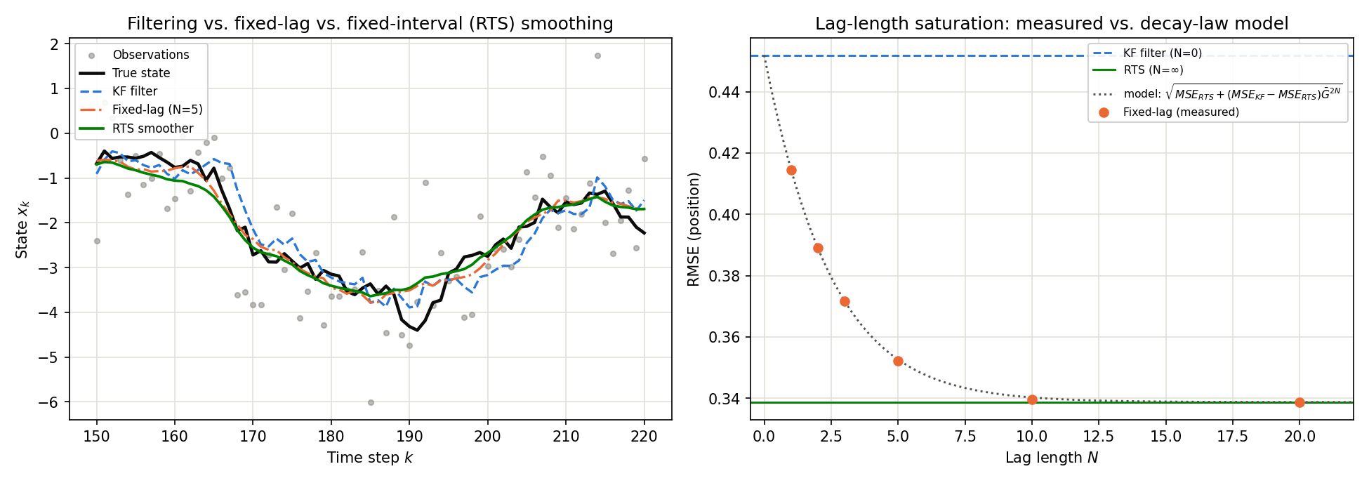
The left panel shows the filter estimate (blue dashed) reacting sharply to observation noise, while the fixed-lag (orange dash-dot) and RTS (green solid) estimates are smoother and track the true state (black) more closely. The right panel shows the measured RMSE (orange dots) sitting almost exactly on the decay-law curve (gray dotted), converging from the filter side toward RTS by \(N \gtrsim 10\) .
Edge Cases: Smoother Behavior Under Degenerate Conditions
Two degenerate conditions are easy to miss from the derivations alone; we check both directly in code.
Edge Case 1: Lag \(N \geq T\) Degenerates Exactly to the Fixed-Interval (RTS) Smoother
The windowed-RTS implementation (Implementation 2) is “the fixed-interval smoother truncated at the window’s endpoint,” so once the window covers the entire record, the fixed-lag estimate must match RTS exactly, numerically.
x_lag_full = fixed_lag_smoother(y_obs, F, H, Q, R, x0, P0, N=T)
x_lag_over = fixed_lag_smoother(y_obs, F, H, Q, R, x0, P0, N=T + 100)
print(f"max |x_lag(N=T)   - x_rts| = {np.max(np.abs(x_lag_full[:, 0] - x_rts[:, 0])):.3e}")
print(f"max |x_lag(N=T+100) - x_rts| = {np.max(np.abs(x_lag_over[:, 0] - x_rts[:, 0])):.3e}")
Output:
max |x_lag(N=T)   - x_rts| = 0.000e+00
max |x_lag(N=T+100) - x_rts| = 0.000e+00
The difference is exactly zero (because j0 = max(0, k - N) pins the window’s left edge to \(0\)
once \(N \geq T\)
, making the windowed-RTS recursion identical, step for step, to the RTS backward recursion). In practice this means setting the lag length larger than the record length is always safe — it silently returns the same result as RTS, with no upper bound to worry about.
Edge Case 2: The \(Q=0\) Limit and a Trap in the Smoother Gain
Substituting \(Q=0\) (no process noise for just this one step) into the smoother gain \(G_k = P_{k|k} F^T P_{k+1|k}^{-1}\) gives \(P_{k+1|k} = F P_{k|k} F^T\) , so
\[ G_k = P_{k|k} F^T (F P_{k|k} F^T)^{-1} = F^{-1} \]— exactly, regardless of the value of \(P_{k|k}\) (assuming \(F\) is invertible). For \(F=1\) (the random walk above) this is trivial, \(G_k=1\) ; a mean-reverting system (say, an AR(1) model with \(F=0.9\) ) gives a non-trivial value.
F_ar, H_ar, R_ar = 0.9, 1.0, 1.0
P = 1.0  # arbitrary initial value (need not be at steady state)
for k in range(8):
    P_pred_val = F_ar**2 * P + 0.0  # Q = 0 exactly
    G_val = P * F_ar / P_pred_val
    print(f"k={k}: P_filt={P:.6e}, G_k={G_val:.6f}  (1/F = {1/F_ar:.6f})")
    S = H_ar**2 * P_pred_val + R_ar
    K = P_pred_val * H_ar / S
    P = (1 - K * H_ar) * P_pred_val
Output:
k=0: P_filt=1.000000e+00, G_k=1.111111  (1/F = 1.111111)
k=1: P_filt=4.475138e-01, G_k=1.111111  (1/F = 1.111111)
k=2: P_filt=2.660476e-01, G_k=1.111111  (1/F = 1.111111)
k=3: P_filt=1.772923e-01, G_k=1.111111  (1/F = 1.111111)
k=4: P_filt=1.255736e-01, G_k=1.111111  (1/F = 1.111111)
k=5: P_filt=9.232390e-02, G_k=1.111111  (1/F = 1.111111)
k=6: P_filt=6.957907e-02, G_k=1.111111  (1/F = 1.111111)
k=7: P_filt=5.335217e-02, G_k=1.111111  (1/F = 1.111111)
Even though \(P_{k|k}\) shrinks monotonically (uncertainty decreases with each observation), \(G_k\) stays pinned exactly at \(1/F=1.1111\ldots\) . This is because the same \(P_{k|k}\) appears in the numerator and denominator and cancels exactly — it is an identity, not an approximation.
There is an important caveat here. Taking “the \(Q \to 0\) limit” via the steady state (the fixed point reached if every \(k\) used the same small \(Q\) ) gives a completely different answer than substituting \(Q=0\) at a single step. For a stable system (\(|F|<1\) ), as \(Q \to 0\) the steady-state covariance \(\bar{P}_{k|k}\) itself shrinks proportionally to \(Q\) (the standard AR(1) approximation \(\bar{P}_{k|k} \approx Q/(1-F^2)\) ), so the ratio \(G_k = \bar{P}_{k|k} F/(F^2\bar{P}_{k|k}+Q)\) becomes a \(0/0\) indeterminate form, converging not to \(1/F\) but to \(F\) itself.
for Qval in [1e-1, 1e-3, 1e-6, 1e-9, 1e-12]:
    P = 1.0
    for _ in range(2000):  # iterate to steady state
        P_pred_val = F_ar**2 * P + Qval
        S = H_ar**2 * P_pred_val + R_ar
        K = P_pred_val * H_ar / S
        P = (1 - K * H_ar) * P_pred_val
    P_pred_val = F_ar**2 * P + Qval
    G_val = P * F_ar / P_pred_val
    print(f"Q={Qval:.0e}: steady-state P_filt={P:.3e}, G_bar={G_val:.8f}")
Output:
Q=1e-01: steady-state P_filt=2.153e-01, G_bar=0.70620719
Q=1e-03: steady-state P_filt=5.124e-03, G_bar=0.89538818
Q=1e-06: steady-state P_filt=5.263e-06, G_bar=0.89999526
Q=1e-09: steady-state P_filt=5.263e-09, G_bar=0.90000000
Q=1e-12: steady-state P_filt=5.263e-12, G_bar=0.90000000
As \(Q\) shrinks, \(G_{\mathrm{bar}}\) converges to \(F=0.9\) — a different value than the \(1/F=1.111\ldots\) obtained by substituting \(Q=0\) at a single step. Substituting \(Q=0\) and taking the steady-state limit \(Q\to0\) do not commute — a classic pitfall of the order in which limits are taken. When reasoning intuitively about smoother-gain behavior for a system with a severely underestimated process-noise variance, this non-commutativity is worth keeping in mind.
Recent Research: Numerically Stabilizing the Fixed-Point Smoother
While research on the fixed-interval (RTS) smoother has stayed active through the 2020s, the fixed-point smoother has long been used with its implementation pitfalls (the cost blow-up from state augmentation, or the numerical instability of a naive implementation of the recursion we derived in equations \((17)\) –\((18)\) ) never fully sorted out. Filling this gap, Krämer (2024/2025), “Numerically Robust Fixed-Point Smoothing Without State Augmentation,” proposes a Cholesky-based formulation of the fixed-point smoother that avoids state augmentation entirely. It sidesteps downdates (subtractive updates to a Cholesky factor that tend to amplify numerical error) while achieving both fast execution and numerical robustness — according to the author, existing implementations had to sacrifice one for the other. Estimating systems with unknown initial conditions is an important practical use case, and the fixed-point smoother has accumulated far less research than the fixed-interval smoother, making this work a genuine gap-filler.
Beyond Linear Gaussian Models
This article was restricted to linear Gaussian systems, but the same three-way classification carries over directly to nonlinear and non-Gaussian settings. Besides EKF/UKF-based smoothers, particle smoothers (forward-filtering backward-smoothing, \(O(T M^2)\) with \(M\) particles) re-weight the samples of a particle filter backward in time, enabling smoothing of multimodal posteriors. More recently, deep state space models (Deep Kalman Filters, the S4/Mamba family) learn the transition and observation models with neural networks, and the same filtering-vs-smoothing distinction reappears in their variational posterior approximations. The latency and complexity intuitions of classical smoothers transfer directly to these modern methods.
Summary
- Smoothing is non-causal estimation that uses future observations: it never does worse than filtering, but it introduces latency
- RTS (fixed-interval) is the offline gold standard for all time steps; fixed-lag trades a delay of \(N\) steps for near-RTS accuracy in streaming settings; fixed-point incrementally refines one specific time step at minimal cost
- The two fixed-lag implementations (state-augmented Kalman filter vs. windowed RTS) were shown to agree numerically to within \(10^{-15}\) , and the fixed-point smoother’s update equations were derived rigorously from a telescoping RTS recursion
- A 50-run Monte Carlo on a random walk confirmed the monotone improvement: filter RMSE 0.4519 → fixed-lag \(N=5\) 0.3521 → RTS 0.3388
- The lag length’s benefit was shown, both by derivation and by measurement, to saturate exponentially in the square of the steady-state smoother gain, \(\bar{G}^{2N}\) (measured vs. predicted RMSE differed by at most \(0.0006\) )
- Substituting \(Q=0\) at a single step gives exactly \(G_k=F^{-1}\) , while the steady-state limit \(Q\to0\) instead converges to \(G_{\mathrm{bar}}\to F\) — a non-commutativity to watch for (measured: \(1/F=1.111\) vs. \(F=0.9\) for a system with \(F=0.9\) )
Related Articles
- Kalman Smoother (Rauch-Tung-Striebel / RTS): Forward-Backward Recursion and Python Implementation - Detailed derivation and implementation of the fixed-interval (RTS) smoother; the prerequisite for this article.
- Kalman Filter: Theory and Python Implementation - The forward pass underlying every smoother in this article.
- Extended Kalman Filter (EKF): Theory and Python Implementation - First step toward nonlinear systems and EKF-based smoothers.
- Unscented Kalman Filter (UKF): Theory and Python Implementation - Sigma-point nonlinear estimation, extensible to UKF smoothers.
- Particle Filter in Python: Comparing Resampling Methods - The foundation for particle smoothers in non-Gaussian systems.
- Nonlinear Kalman Smoothers (EKS/URTS) - The follow-up article: implements the EKF/UKF-based smoothers mentioned at the end of this article and compares their accuracy on a strongly nonlinear benchmark.
References
- Rauch, H. E., Tung, F., & Striebel, C. T. (1965). “Maximum likelihood estimates of linear dynamic systems.” AIAA Journal, 3(8), 1445-1450.
- Bryson, A. E., & Frazier, M. (1963). “Smoothing for linear and nonlinear dynamic systems.” Proceedings of the Optimum System Synthesis Conference, 353-364.
- Biswas, K. K., & Mahalanabis, A. K. (1972). “An approach to fixed-lag smoothing problems.” IEEE Transactions on Aerospace and Electronic Systems, AES-8(5), 676-682.
- Meditch, J. S. (1969). Stochastic Optimal Linear Estimation and Control. McGraw-Hill.
- Anderson, B. D. O., & Moore, J. B. (1979). Optimal Filtering. Prentice-Hall.
- Särkkä, S. (2013). Bayesian Filtering and Smoothing. Cambridge University Press.
- Krämer, N. (2024/2025). “Numerically Robust Fixed-Point Smoothing Without State Augmentation.” arXiv:2409.20004.