Introduction: Why Block DCT Produces Boundary Artifacts
The Discrete Cosine Transform (DCT) has excellent energy compaction, and the 8×8 block DCT is the workhorse of JPEG. However, when a signal is split into non-overlapping blocks that are transformed and quantized independently, reconstruction errors stay confined within each block while nothing guarantees continuity across neighboring blocks. Quantization error therefore shows up as discontinuities at block boundaries. In images this is the familiar JPEG blocking noise; in audio, per-boundary discontinuities are perceived as periodic clicks (blocking artifacts) and are far more objectionable to the ear.
The natural remedy is to overlap the frames. But a naive 50%-overlapped DCT produces \(2M\) coefficients every \(M\) samples, so the representation becomes 2x redundant — a non-starter when the goal is compression.
The MDCT (Modified Discrete Cosine Transform) reconciles “smoothness from overlap” with “critical sampling (number of coefficients = number of input samples)”. By deliberately producing only \(M\) coefficients from \(2M\) input samples, the total coefficient count matches the sample count even with 50% overlap. The time-domain aliasing introduced by halving the output is exactly cancelled by overlap-add with the neighboring frames. This mechanism is TDAC (Time-Domain Aliasing Cancellation).
The MDCT is used in essentially all modern audio codecs: MP3 (as the second stage of its hybrid filter bank), AAC, Vorbis, Opus (the CELT layer), and AC-3. In this article we derive the MDCT definition and the TDAC mechanism, work through the perfect-reconstruction window condition (the Princen-Bradley condition) and the cosine-modulated filter bank interpretation, then numerically verify perfect reconstruction with a from-scratch numpy implementation and run a boundary-artifact experiment against block DCT.
Definition of the MDCT and TDAC
Forward and Inverse Transforms
For a frame \(x[n]\) of length \(2M\) (\(n = 0, \ldots, 2M-1\) ) and a window \(w[n]\) , the MDCT outputs \(M\) coefficients:
\[ X[k] = \sum_{n=0}^{2M-1} w[n]\, x[n] \cos\left(\frac{\pi}{M}\left(n + \frac{1}{2} + \frac{M}{2}\right)\left(k + \frac{1}{2}\right)\right), \quad k = 0, \ldots, M-1 \tag{1} \]The inverse MDCT (IMDCT) maps \(M\) coefficients back to a length-\(2M\) signal:
\[ \hat{x}[n] = \frac{2}{M}\, w[n] \sum_{k=0}^{M-1} X[k] \cos\left(\frac{\pi}{M}\left(n + \frac{1}{2} + \frac{M}{2}\right)\left(k + \frac{1}{2}\right)\right) \tag{2} \]With \(2M\) inputs and only \(M\) outputs, a single frame loses half its information and cannot be inverted on its own: the map \(2M \to M\) is singular with an \(M\) -dimensional kernel. This is fundamentally different from the DCT-II, an \(N \to N\) orthogonal transform that is invertible by itself.
Applying equation \((1)\) with hop size \(M\) (50% overlap) yields \(M\) coefficients per \(M\) samples — critical sampling.
The Structure of Time-Domain Aliasing
Where did the missing half of the information go? Write the frame as four quarters of length \(M/2\) , \(x = (a, b, c, d)\) , and let \(R(\cdot)\) denote time reversal. Without a window (\(w[n] = 1\) ) the following identity holds:
\[ \text{IMDCT}(\text{MDCT}(x)) = \bigl(a - R(b),\; b - R(a),\; c + R(d),\; d + R(c)\bigr) \tag{3} \]A single-frame reconstruction is thus the original signal contaminated by time-reversed folded components (time-domain aliasing). The key point is that the first half folds with odd symmetry (\(-R\) ) and the second half with even symmetry (\(+R\) ). This is the time/frequency dual of the familiar fact from multirate signal processing that decimation creates (frequency-domain) aliasing.
TDAC: Cancellation via Overlap-Add
The second half \((c, d)\) of frame \(i\) is transformed again as the first half \((a', b') = (c, d)\) of frame \(i+1\) . By equation \((3)\) , the same interval is reconstructed as
- from frame \(i\) : \(c + R(d)\) , \(d + R(c)\) (even-symmetric folding)
- from frame \(i+1\) : \(c - R(d)\) , \(d - R(c)\) (odd-symmetric folding)
Adding the two, the aliasing terms \(\pm R(\cdot)\) cancel exactly with opposite signs, leaving \(2c\) , \(2d\) (the factor \(2/M\) in equation \((2)\) absorbs this doubling into the normalization). This is the essence of TDAC: although a single frame is unrecoverable, each frame carries the antidote to its neighbor’s aliasing, so perfect reconstruction holds after overlap-add (OLA).
With a window \(w[n]\) , the same window is applied twice (analysis and synthesis), so cancellation reduces to a symmetry requirement plus an amplitude condition on the window — the Princen-Bradley condition of the next section.
Perfect Reconstruction Conditions on the Window
The Princen-Bradley Condition
For a symmetric window \(w[2M-1-n] = w[n]\) , the overlap-added amplitude equals 1 at every sample if and only if
\[ w[n]^2 + w[n+M]^2 = 1, \quad n = 0, \ldots, M-1 \tag{4} \](the Princen-Bradley condition). Sketch of the derivation: inserting the window into equation \((3)\) , each sample \(n\) in the overlap region picks up (i) a factor \(w[n+M]^2 + w[n]^2\) on the signal component, and (ii) a factor \(w[n+M]\,w_R[n+M] - w[n]\,w_R[n]\) on the aliasing component. If the window is symmetric, (ii) vanishes identically so the aliasing cancels, and if (i) satisfies equation \((4)\) the amplitude is preserved as well. This plays the same role as the STFT’s COLA condition (\(\sum w = \text{const}\) ) covered in Spectrogram in Practice , but because the window is applied twice in the MDCT, the condition involves the sum of squared windows.
The Sine Window
The simplest window satisfying equation \((4)\) is the sine window:
\[ w[n] = \sin\left(\frac{\pi}{2M}\left(n + \frac{1}{2}\right)\right), \quad n = 0, \ldots, 2M-1 \tag{5} \]Equation \((4)\) follows immediately from \(\sin^2\theta + \cos^2\theta = 1\) . It is used in MP3 and Vorbis, and the MDCT with this window coincides with Malvar’s MLT (Modulated Lapped Transform).
The KBD Window
The KBD (Kaiser-Bessel Derived) window is built as the square root of the cumulative sum of a Kaiser window \(v[j]\) of length \(M+1\) :
\[ w[n] = \sqrt{\frac{\sum_{j=0}^{n} v[j]}{\sum_{j=0}^{M} v[j]}}, \quad n = 0, \ldots, M-1 \tag{6} \](the second half is mirrored). The square-root-of-cumulative-sum construction satisfies equation \((4)\) automatically. Compared with the sine window it has a wider main lobe but much stronger stopband attenuation; AAC switches between the sine and KBD windows depending on the signal. The Kaiser parameter \(\alpha\) trades leakage against resolution, exactly the same design intuition as STFT window selection.
The MDCT as a Filter Bank
Cosine-Modulated Filter Bank
The MDCT is simultaneously a transform and an \(M\) -band critically sampled perfect-reconstruction filter bank. Equation \((1)\) is equivalent to convolving the signal with analysis filters of length \(2M\) ,
\[ h_k[n] = w[n] \cos\left(\frac{\pi}{M}\left(n + \frac{1}{2} + \frac{M}{2}\right)\left(k + \frac{1}{2}\right)\right) \tag{7} \]and downsampling the outputs by \(M\) . Each \(h_k\) is a single prototype (lowpass) window \(w[n]\) cosine-modulated to center frequency \(\omega_k = \frac{\pi}{M}\left(k + \frac{1}{2}\right)\) , which is why the MDCT is classified as a cosine-modulated filter bank: \(M\) bandpass filters uniformly partition the Nyquist band and each band is sampled at rate \(1/M\) — precisely the decimation framework of multirate signal processing .
Each band on its own is full of aliasing (the filter transition bands overlap heavily with neighboring bands), yet summing all bands on the synthesis side cancels the aliasing — this is TDAC restated in the frequency domain.
Polyphase Representation and Fast Computation
With filter length \(2M\) and decimation factor \(M\) , the polyphase decomposition has only 2 taps per polyphase component. This structure lets the MDCT be computed in two stages:
- Windowing + folding: fold the \(2M\) windowed samples down to \(M\) using the symmetries of equation \((3)\) (\(O(M)\) )
- DCT-IV: apply a DCT-IV to the folded \(M\) points (\(O(M \log M)\) via FFT)
The fact that the MDCT is “a DCT-IV with a windowing-and-folding pre-stage” is the practical key that reduces the naive \(O(M^2)\) matrix product to \(O(M \log M)\) . Historically, MP3 uses a hybrid of a 32-band PQMF (pseudo-QMF filter bank) followed by an 18-point MDCT, while AAC and later codecs use a single MDCT (window switching between \(M = 1024/128\) ).
Python Implementation: MDCT/IMDCT and Numerical Verification of Perfect Reconstruction
Windows and the Princen-Bradley Condition
We build the KBD window from a Kaiser window generated with scipy.signal.get_window, following equation \((6)\)
.
import numpy as np
from scipy.signal import get_window

def sine_window(N):
    """Sine window: the simplest window satisfying the Princen-Bradley condition"""
    n = np.arange(N)
    return np.sin(np.pi / N * (n + 0.5))

def kbd_window(N, alpha=4.0):
    """Kaiser-Bessel Derived (KBD) window: used in AAC"""
    M = N // 2
    kaiser = get_window(("kaiser", np.pi * alpha), M + 1, fftbins=False)
    csum = np.cumsum(kaiser)
    half = np.sqrt(csum[:M] / csum[M])
    return np.concatenate([half, half[::-1]])

# Verify the Princen-Bradley condition w_n^2 + w_{n+M}^2 = 1
N = 512
for name, w in [("sine", sine_window(N)), ("KBD (alpha=4)", kbd_window(N))]:
    err = np.max(np.abs(w[: N // 2] ** 2 + w[N // 2 :] ** 2 - 1.0))
    print(f"{name:14s}: max |w_n^2 + w_(n+M)^2 - 1| = {err:.2e}")
sine          : max |w_n^2 + w_(n+M)^2 - 1| = 4.44e-16
KBD (alpha=4) : max |w_n^2 + w_(n+M)^2 - 1| = 5.55e-16
Both windows satisfy the Princen-Bradley condition to machine precision.
The MDCT/IMDCT Core
We implement equations \((1)\) and \((2)\) directly as matrix products (for clarity; production code would use folding + DCT-IV from the previous section).
def mdct(frame, w):
    """MDCT of one frame: M coefficients from a length-2M input (eq. 1)"""
    N = len(frame)
    M = N // 2
    n = np.arange(N)
    k = np.arange(M)
    C = np.cos(np.pi / M * (n[None, :] + 0.5 + M / 2) * (k[:, None] + 0.5))
    return C @ (w * frame)

def imdct(X, w):
    """Inverse MDCT of one frame: length-2M signal from M coefficients (eq. 2)"""
    M = len(X)
    n = np.arange(2 * M)
    k = np.arange(M)
    C = np.cos(np.pi / M * (n[:, None] + 0.5 + M / 2) * (k[None, :] + 0.5))
    return (2.0 / M) * w * (C @ X)

def mdct_analysis(x, w):
    """MDCT coefficients of all frames with hop M (50% overlap)"""
    N = len(w)
    M = N // 2
    n_frames = len(x) // M - 1
    return np.stack([mdct(x[i * M : i * M + N], w) for i in range(n_frames)])

def mdct_synthesis(coeffs, w, length):
    """Reconstruct the signal via inverse MDCT + overlap-add (OLA)"""
    n_frames, M = coeffs.shape
    y = np.zeros(length)
    for i in range(n_frames):
        y[i * M : i * M + 2 * M] += imdct(coeffs[i], w)
    return y
Verifying the TDAC Identity
We directly check the aliasing structure of equation \((3)\) on a single unwindowed frame.
rng = np.random.default_rng(42)
M = 8
x = rng.standard_normal(2 * M)
y_single = imdct(mdct(x, np.ones(2 * M)), np.ones(2 * M))  # no window

h = M // 2
a, b, c, d = x[:h], x[h : 2 * h], x[2 * h : 3 * h], x[3 * h :]
R = lambda v: v[::-1]
tdac_expected = np.concatenate([a - R(b), b - R(a), c + R(d), d + R(c)])
print(f"TDAC identity verification error: {np.max(np.abs(y_single - tdac_expected)):.2e}")
TDAC identity verification error: 6.00e-15
The single-frame reconstruction is indeed of the aliased form \((a - R(b),\ b - R(a),\ c + R(d),\ d + R(c))\) ; equation \((3)\) holds to machine precision.
Visualizing TDAC: Single-Frame Reconstruction vs. Overlap-Add
Having confirmed identity \((3)\) algebraically on a tiny \(M=8\) example, we now visualize the same phenomenon as waveforms on a windowed, multi-frame signal: how far a single-frame reconstruction strays from the original, and how completely overlap-add (OLA) cancels that error. With an \(M=64\) sine window on a smooth signal made of two sinusoids, we compare (i) reconstructing frame 3 alone via IMDCT against (ii) reconstructing the whole signal via OLA over all frames.
import matplotlib.pyplot as plt

M = 64
w = sine_window(2 * M)
n_idx = np.arange(9 * M)
x = np.sin(2 * np.pi * 5 * n_idx / (9 * M)) + 0.5 * np.sin(
    2 * np.pi * 13 * n_idx / (9 * M) + 0.3
)

coeffs = mdct_analysis(x, w)
y_full = mdct_synthesis(coeffs, w, len(x))

# Reconstruct frame 3 alone (no OLA with neighboring frames)
fi = 3
y_single = np.full(len(x), np.nan)
y_single[fi * M : fi * M + 2 * M] = imdct(coeffs[fi], w)

# Compare error in the overlap region shared by frame 3 and frame 4
ov_lo, ov_hi = (fi + 1) * M, (fi + 2) * M
target = w[M:] * x[ov_lo:ov_hi]
e_alias = np.max(np.abs(y_single[ov_lo:ov_hi] - target))
e_recon = np.max(np.abs(y_full[M:-M] - x[M:-M]))
print(f"aliasing error, single frame (no OLA): {e_alias:.4f}")
print(f"perfect reconstruction error after OLA: {e_recon:.2e}")
aliasing error, single frame (no OLA): 0.7346
perfect reconstruction error after OLA: 3.71e-14
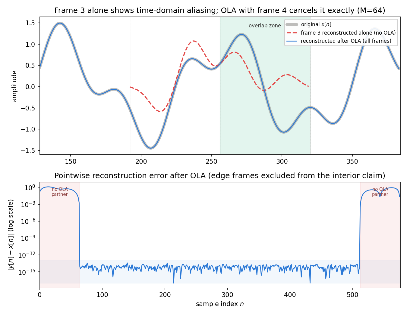
As the figure shows, reconstructing frame 3 alone via IMDCT (red dashed) drifts increasingly far from the original (thick gray) moving into the second half of the overlap region — this is exactly the time-domain aliasing of equation \((3)\) . Reconstruction after OLA with the neighboring frame (blue), by contrast, overlays the original almost perfectly. Numerically, the overlap-region error for the isolated reconstruction peaked at \(0.7346\) (on the same order as the signal amplitude), while after OLA it dropped to \(3.71 \times 10^{-14}\) — an improvement by a factor of roughly \(2 \times 10^{13}\) . This makes concrete, at the waveform level, TDAC’s claim that “each frame carries the antidote to its neighbor’s aliasing.” The bottom error panel shows the OLA error pinned to a noise floor around \(10^{-15}\) throughout the interior, jumping up to the signal’s own amplitude only at the first and last \(M\) samples, which have no OLA partner.
Numerical Verification of Perfect Reconstruction
We measure the analysis-synthesis round-trip error on random signals generated with numpy.random.default_rng.
for M in [32, 64, 256, 512]:
    L = 64 * M
    x = rng.standard_normal(L)
    for name, w in [("sine", sine_window(2 * M)), ("KBD ", kbd_window(2 * M))]:
        coeffs = mdct_analysis(x, w)
        y = mdct_synthesis(coeffs, w, L)
        err = np.max(np.abs(x[M:-M] - y[M:-M]))  # first/last M samples have no OLA partner
        print(f"M={M:4d}, {name} window: perfect reconstruction error = {err:.2e}")
M=  32, sine window: perfect reconstruction error = 3.77e-14
M=  32, KBD  window: perfect reconstruction error = 3.54e-14
M=  64, sine window: perfect reconstruction error = 6.75e-14
M=  64, KBD  window: perfect reconstruction error = 6.57e-14
M= 256, sine window: perfect reconstruction error = 3.39e-13
M= 256, KBD  window: perfect reconstruction error = 3.30e-13
M= 512, sine window: perfect reconstruction error = 6.59e-13
M= 512, KBD  window: perfect reconstruction error = 7.28e-13
The reconstruction error is on the order of \(10^{-14}\) to \(10^{-13}\) — i.e. double-precision machine precision (each coefficient is an inner product of length \(2M\) , so rounding error accumulates mildly as \(O(M)\) , giving a few hundred times \(\varepsilon \approx 10^{-16}\) ). TDAC-based perfect reconstruction is confirmed numerically: without quantization, the MDCT loses not a single bit — a critically sampled and invertible representation. Note that the first and last \(M\) samples have no overlap partner, so cancellation does not occur there; this is exactly why practical codecs incur one frame of algorithmic delay (look-ahead).
Experiment: Block DCT vs MDCT on a Chirp Signal
To expose the boundary-artifact difference, we apply a simple compression model — “keep only the top \(p\%\)
of coefficients by magnitude, zero out the rest” — to a chirp (200→3000 Hz) plus a steady tone, comparing a non-overlapping block DCT (scipy.fft.dct) and the MDCT at the same block size \(M = 256\)
.
from scipy.fft import dct, idct

fs = 8000
t = np.arange(fs) / fs                              # 1 second
sig = np.sin(2 * np.pi * (200 * t + 1400 * t**2))   # 200 -> 3000 Hz chirp
sig += 0.3 * np.sin(2 * np.pi * 440 * t)            # steady tone

M = 256
w = sine_window(2 * M)
L = len(sig)
pad = M  # padding for OLA at both ends
xpad = np.concatenate([np.zeros(pad), sig, np.zeros(pad + (-(L + 2 * pad)) % M)])

def keep_top(coeffs, ratio):
    """Keep only the top `ratio` fraction of coefficients by magnitude"""
    flat = np.abs(coeffs).ravel()
    thr = np.sort(flat)[::-1][int(flat.size * ratio) - 1]
    return np.where(np.abs(coeffs) >= thr, coeffs, 0.0)

nblk = L // M
sd = sig[: nblk * M]
for ratio in [0.10, 0.05]:
    # MDCT (50% overlap, critically sampled)
    cm = keep_top(mdct_analysis(xpad, w), ratio)
    ym = mdct_synthesis(cm, w, len(xpad))[pad : pad + L]
    snr_m = 10 * np.log10(np.sum(sig**2) / np.sum((sig - ym) ** 2))
    # Non-overlapping block DCT (same block size M)
    cd = keep_top(dct(sd.reshape(nblk, M), type=2, norm="ortho", axis=1), ratio)
    yd = idct(cd, type=2, norm="ortho", axis=1).ravel()
    snr_d = 10 * np.log10(np.sum(sd**2) / np.sum((sd - yd) ** 2))
    # Separate error near block boundaries (8 samples at each block edge) vs interior
    idx = np.arange(len(sd))
    near = (idx % M < 8) | (idx % M >= M - 8)
    ed, em = np.abs(sd - yd), np.abs(sig - ym)[: nblk * M]
    print(f"coefficients kept: {ratio*100:.0f}%")
    print(f"  block DCT: SNR {snr_d:5.2f} dB | "
          f"boundary RMS {np.sqrt(np.mean(ed[near]**2)):.4f} / interior RMS {np.sqrt(np.mean(ed[~near]**2)):.4f}")
    print(f"  MDCT     : SNR {snr_m:5.2f} dB | "
          f"boundary RMS {np.sqrt(np.mean(em[near]**2)):.4f} / interior RMS {np.sqrt(np.mean(em[~near]**2)):.4f}")
coefficients kept: 10%
  block DCT: SNR 17.88 dB | boundary RMS 0.3096 / interior RMS 0.0560
  MDCT     : SNR 37.94 dB | boundary RMS 0.0191 / interior RMS 0.0079
coefficients kept: 5%
  block DCT: SNR 13.39 dB | boundary RMS 0.4551 / interior RMS 0.1140
  MDCT     : SNR 23.80 dB | boundary RMS 0.0708 / interior RMS 0.0433
The results are clear-cut:
- SNR: with 10% of coefficients kept, the MDCT is about 20 dB better (37.94 dB vs 17.88 dB)
- Boundary artifacts: for block DCT, the RMS error over the 8 samples at each block edge is 5.5x the interior value (0.3096 vs 0.0560), i.e. the error concentrates at boundaries. For MDCT the boundary/interior ratio stays around 2.4x and is an order of magnitude smaller in absolute terms
With block DCT, the chirp’s instantaneous frequency varies within each block, so truncation-induced discontinuities are exposed at the boundaries; the MDCT’s windowing plus overlap absorbs them smoothly.
Coefficient Sparsity
We also compare energy compaction of the coefficients on the same signal.
cm = mdct_analysis(xpad, w)
cd = dct(sd.reshape(nblk, M), type=2, norm="ortho", axis=1)
for name, cc in [("MDCT", cm), ("block DCT", cd)]:
    e = np.sort((cc**2).ravel())[::-1]
    frac = np.cumsum(e) / np.sum(e)
    n99 = np.searchsorted(frac, 0.99) + 1
    print(f"{name}: coefficients needed for 99% energy: {n99}/{frac.size} ({n99/frac.size*100:.1f}%)")
MDCT: coefficients needed for 99% energy: 364/8448 (4.3%)
block DCT: coefficients needed for 99% energy: 1090/7936 (13.7%)
The MDCT captures 99% of the energy with 4.3% of the coefficients, versus 13.7% for the block DCT. Because the window tapers each frame smoothly to zero, there is no spectral leakage from rectangular truncation and the coefficients are sparser — this is why audio codecs keep choosing the MDCT.
Comparison: DCT / STFT / MDCT / Wavelet Packets
Positioning these time-frequency representations side by side, with hop size \(H\) and window/frame length \(N_w\) :
| Aspect | Block DCT | STFT | MDCT | Wavelet packets |
|---|---|---|---|---|
| Redundancy | 1x (critical) | \(N_w/H\) (2x at 50% overlap) | 1x (critical) | 1x (orthogonal basis) |
| Overlap | none | yes (COLA condition) | yes (TDAC) | depends on filter length |
| Perfect reconstruction | yes (without quantization) | yes (under NOLA/COLA) | yes (under Princen-Bradley) | yes (orthogonal wavelets) |
| Boundary artifacts | yes (quantization error exposed) | rare | rare | depends on boundary handling |
| Algorithmic delay | \(M\) | \(N_w\) | \(2M\) (one frame look-ahead) | depth × filter length |
| Frequency splitting | uniform, \(M\) bands | uniform | uniform, \(M\) bands | adaptive (non-uniform possible) |
| Phase information | none (real coefficients) | yes (complex) | none (real coefficients) | none (real coefficients) |
| Typical use | JPEG, video intra coding | analysis, speech enhancement, phase editing | audio coding (MP3/AAC/Opus) | adaptive bases, features, denoising |
Rules of thumb:
- Compression (minimizing bits) → the critically sampled MDCT: it gives up phase in exchange for critical sampling plus smooth reconstruction
- Analysis and editing (looking at spectrograms, manipulating phase) → the redundant, complex STFT; the parameter design from Spectrogram in Practice applies directly
- Non-uniform frequency splitting (mixed transients and steady tones) → wavelet packets with best-basis selection
Beyond the Classics: MDCT in Neural Audio Codecs
The MDCT is not confined to classical waveform codecs like MP3/AAC/Opus — it has also been adopted in recent neural audio codecs. MDCTCodec (Jiang et al., 2024, arXiv:2411.00464), presented at the 2024 IEEE Spoken Language Technology Workshop (SLT 2024), uses the MDCT spectrum, rather than the STFT spectrogram, as the input and output representation of an end-to-end neural codec: the encoder maps it to a continuous latent representation, which is discretized by residual vector quantization (RVQ), and the decoder reconstructs the waveform via inverse MDCT. Training uses adversarial learning with a multi-resolution MDCT-based discriminator (MR-MDCTD) that distinguishes natural from decoded MDCT spectra. Because MDCT coefficients are real-valued and critically sampled — unlike the STFT — the representation is more compact, and the codec achieves a ViSQOL score of 4.18 at a high sampling rate / low bitrate operating point of 48 kHz and 6 kbps, while also reducing model size and training cost.
The sparsity we measured in this article (block DCT needs 13.7% of coefficients for 99% of the energy, MDCT only 4.3%) is exactly the property that makes the MDCT an efficient input representation for a neural network. It is a striking example of a roughly 40-year-old classical result — TDAC — still shaping design decisions (why choose MDCT over STFT) in modern learning-based audio codecs.
Summary
- Block DCT is critically sampled but exposes quantization error at block boundaries; naive overlap doubles the redundancy. The MDCT, a \(2M \to M\) lapped transform, achieves overlap and critical sampling simultaneously
- A single-frame IMDCT contains time-domain aliasing \((a - R(b),\ b - R(a),\ c + R(d),\ d + R(c))\) , which is exactly cancelled by overlap-add with neighboring frames (TDAC). At the waveform level, the overlap-region error of \(0.7346\) for an isolated frame reconstruction dropped to \(3.71 \times 10^{-14}\) after OLA — an improvement of roughly \(2 \times 10^{13}\) -fold, made visible directly in the figure
- The window condition for perfect reconstruction is the Princen-Bradley condition \(w_n^2 + w_{n+M}^2 = 1\) ; the sine and KBD windows satisfy it, and the numpy implementation reconstructed to \(10^{-14}\) –\(10^{-13}\) (machine precision)
- The MDCT is a cosine-modulated filter bank with the window as prototype; polyphase components have 2 taps, and the practical implementation is “folding + DCT-IV” in \(O(M \log M)\)
- In the 10%-coefficient chirp experiment, block DCT scored SNR 17.9 dB with boundary error 5.5x the interior, while the MDCT scored 37.9 dB with no boundary concentration; coefficients needed for 99% energy dropped from 13.7% to 4.3%, so the MDCT also wins on sparsity
- This sparsity is not just an implementation nicety: 2024’s MDCTCodec (Jiang et al., arXiv:2411.00464) exploits it as the input representation for a neural audio codec
Related Articles
- Discrete Cosine Transform (DCT): Theory and Python Implementation — DCT-II definition, energy compaction, and JPEG; the block-transform foundation for this article.
- Multirate Signal Processing: Theory and Python Implementation — decimation, polyphase decomposition, and Noble identities; the basis for the filter-bank view of the MDCT.
- Short-Time Fourier Transform (STFT): Theory and Python Implementation — the complex-valued counterpart sharing the overlap/window/inverse structure of the MDCT.
- Spectrogram in Practice — STFT Parameter Design — COLA/NOLA conditions and window design in practice; useful to contrast with the Princen-Bradley condition.
- Wavelet Packet Transform and Best Basis Selection — an orthogonal transform achieving adaptive non-uniform frequency splitting, versus the MDCT’s uniform bands.
References
- Princen, J. P., & Bradley, A. B. (1986). “Analysis/synthesis filter bank design based on time domain aliasing cancellation.” IEEE Transactions on Acoustics, Speech, and Signal Processing, 34(5), 1153-1161.
- Princen, J. P., Johnson, A. W., & Bradley, A. B. (1987). “Subband/transform coding using filter bank designs based on time domain aliasing cancellation.” Proc. IEEE ICASSP, 2161-2164.
- Malvar, H. S. (1992). Signal Processing with Lapped Transforms. Artech House.
- Bosi, M., & Goldberg, R. E. (2003). Introduction to Digital Audio Coding and Standards. Springer.
- Vaidyanathan, P. P. (1993). Multirate Systems and Filter Banks. Prentice Hall.
- Jiang, X.-H., Ai, Y., Zheng, R.-C., Du, H.-P., Lu, Y.-X., & Ling, Z.-H. (2024). “MDCTCodec: A Lightweight MDCT-based Neural Audio Codec towards High Sampling Rate and Low Bitrate Scenarios.” Proc. IEEE Spoken Language Technology Workshop (SLT). arXiv:2411.00464