Introduction
Computing the autocorrelation function (ACF) tells you, lag by lag, how similar a time series is to its own past. But the ACF alone cannot answer this question: “Is the correlation at lag 2 a genuinely direct effect of lag 2, or is it just the lag-1 influence propagating over two steps?”
The tool that answers it is the partial autocorrelation function (PACF). Because the PACF measures the “pure” correlation after removing the influence of intermediate lags, the order \(p\) of an AR model shows up directly as the largest lag at which the PACF is nonzero. This property is the theoretical justification for staring at ACF/PACF plots when choosing orders for an ARIMA model .
This article is the advanced companion to the autocorrelation basics post. We derive the PACF definition (correlation of linear-prediction residuals), the Yule-Walker equations, and the Levinson-Durbin recursion; organize the AR/MA order-identification decision table; and review the AIC/BIC information criteria. Then, using statsmodels (pacf, plot_acf/plot_pacf, levinson_durbin, AutoReg, ar_select_order, arma_order_select_ic, ARIMA), we run numerical experiments on a known AR(2) process and confirm that the “PACF cutoff” and “AIC/BIC minimization” point to the same order.
Definition of the Partial Autocorrelation (PACF)
As a correlation of linear-prediction residuals
For a stationary time series \(\{x_t\}\) , the partial autocorrelation at lag \(k\) is defined as the correlation remaining after the linear effect of the intermediate values \(x_{t-1}, \ldots, x_{t-k+1}\) has been removed from both sides:
\[\alpha(k) = \operatorname{Corr}\left(x_t - \hat{x}_t^{(k-1)},\; x_{t-k} - \hat{x}_{t-k}^{(k-1)}\right) \tag{1}\]Here \(\hat{x}_t^{(k-1)}\) is the best linear prediction of \(x_t\) from \(x_{t-1}, \ldots, x_{t-k+1}\) , and \(\hat{x}_{t-k}^{(k-1)}\) is the best (backward) linear prediction of \(x_{t-k}\) from the same intermediate values. In other words, the PACF is the correlation between the residuals left over after subtracting whatever the intermediate lags can explain—the time-series analogue of the partial correlation coefficient in regression analysis.
As the last coefficient of an AR regression
There is an equivalent second definition. Fit an autoregression of order \(k\) ,
\[x_t = \phi_{k1} x_{t-1} + \phi_{k2} x_{t-2} + \cdots + \phi_{kk} x_{t-k} + \varepsilon_t \tag{2}\]then the last coefficient \(\phi_{kk}\) is exactly the partial autocorrelation at lag \(k\) :
\[\alpha(k) = \phi_{kk} \tag{3}\]It measures “how much additional explanatory power \(x_{t-k}\) has even when lags \(1\) through \(k-1\) are already in the regression,” so intuitively it is the same quantity as equation \((1)\) . Note that \(\alpha(1)\) equals the ordinary autocorrelation \(\rho_1\) , since there are no intermediate lags to remove.
Why the PACF cuts off for AR processes
Consider an AR(1) process \(x_t = \phi x_{t-1} + \varepsilon_t\) . Its ACF decays exponentially as \(\rho_k = \phi^k\) , so even at lag 2 we have \(\rho_2 = \phi^2 \neq 0\) . But that correlation is merely an indirect effect propagated along “\(x_{t-2} \to x_{t-1} \to x_t\) .” Once the effect of \(x_{t-1}\) is removed, no direct contribution of \(x_{t-2}\) remains, hence \(\alpha(2) = 0\) .
In general, for an AR(p) process \(x_t\) is determined by its \(p\) most recent values only (\(\phi_{kk} = 0\) in equation \((2)\) for \(k > p\) ), so
\[\alpha(k) = 0 \quad (k > p) \tag{4}\]The PACF cuts off after lag \(p\) —this is the heart of AR order identification. We give the rigorous proof of this intuition after deriving the Levinson-Durbin recursion (see “Corollary: a rigorous proof of the PACF cutoff” below).
The Yule-Walker Equations
Computing the PACF in practice requires the coefficients \(\phi_{kj}\) of equation \((2)\) . For the AR(p) process
\[x_t = \phi_1 x_{t-1} + \cdots + \phi_p x_{t-p} + \varepsilon_t, \quad \varepsilon_t \sim \mathrm{WN}(0, \sigma^2) \tag{5}\]multiply both sides by \(x_{t-k}\) (\(k \geq 1\) ) and take expectations. Since \(E[\varepsilon_t x_{t-k}] = 0\) , we obtain a linear system in the autocorrelations \(\rho_k\) :
\[\rho_k = \phi_1 \rho_{k-1} + \phi_2 \rho_{k-2} + \cdots + \phi_p \rho_{k-p}, \quad k = 1, \ldots, p \tag{6}\]These are the Yule-Walker equations. Collecting \(k = 1, \ldots, p\) in matrix form,
\[ \begin{pmatrix} 1 & \rho_1 & \cdots & \rho_{p-1} \\ \rho_1 & 1 & \cdots & \rho_{p-2} \\ \vdots & \vdots & \ddots & \vdots \\ \rho_{p-1} & \rho_{p-2} & \cdots & 1 \end{pmatrix} \begin{pmatrix} \phi_1 \\ \phi_2 \\ \vdots \\ \phi_p \end{pmatrix} = \begin{pmatrix} \rho_1 \\ \rho_2 \\ \vdots \\ \rho_p \end{pmatrix} \tag{7} \]The matrix on the left is a Toeplitz matrix, constant along its diagonals. Plugging the sample ACF into equation \((7)\) and solving gives the Yule-Walker estimates of the AR coefficients; solving it for increasing orders \(k = 1, 2, 3, \ldots\) and collecting the last coefficient \(\phi_{kk}\) at each order yields the sample PACF.
The Levinson-Durbin Recursion
Solving equation \((7)\) independently at each order \(k\) repeats an \(O(k^3)\) matrix inversion. The Levinson-Durbin recursion exploits the Toeplitz structure to update the order-\((k-1)\) solution to the order-\(k\) solution in \(O(k)\) .
Deriving the recursion (forward and backward prediction errors)
Rather than accepting equations \((8)\) –\((10)\) below as given, we derive them from the projections of two quantities: the forward prediction error and the backward prediction error.
Let the order-\(k\) forward prediction residual be \(e_k(t) = x_t - \hat{x}_t^{(k)}\) , and define the backward prediction residual as
\[ r_k(t) = x_{t-k-1} - \hat{x}_{t-k-1}^{(k)} \tag{8a} \](the backward prediction regresses \(x_{t-k-1}\) on \(x_{t-k}, \ldots, x_{t-1}\) —a regression run backward in time). Because the autocorrelation matrix of a stationary process is a symmetric Toeplitz matrix, its persymmetry (symmetry about the anti-diagonal) implies that the backward regression coefficients are exactly the forward coefficients \(\phi_{k1}, \ldots, \phi_{kk}\) in reverse order. Consequently, the forward and backward residuals share the same variance \(\sigma_k^2\) .
When the order is raised from \(k\) to \(k+1\) , the new forward error takes the form of a lattice filter: subtract, from the existing forward error, the information carried by the backward error one step earlier.
\[ e_{k+1}(t) = e_k(t) - \phi_{k+1,k+1}\, r_k(t-1) \tag{8b} \] \[ r_{k+1}(t) = r_k(t-1) - \phi_{k+1,k+1}\, e_k(t) \tag{8c} \](Equation \((8b)\) says: use the newly available information \(r_k(t-1)\) about \(x_{t-k-1}\) to further explain \(e_k(t)\) ; equation \((8c)\) is its mirror image.) The new coefficient \(\phi_{k+1,k+1}\) is chosen so that the updated forward error \(e_{k+1}(t)\) is uncorrelated with the newly added information \(r_k(t-1)\) :
\[ \phi_{k+1,k+1} = \frac{E[e_k(t)\, r_k(t-1)]}{E[r_k(t-1)^2]} = \frac{E[e_k(t)\, r_k(t-1)]}{\sigma_k^2} \tag{8d} \]This is exactly the PACF definition, equation \((1)\) : since \(e_k(t) = x_t - \hat{x}_t^{(k)}\) and \(r_k(t-1) = x_{t-k-1} - \hat{x}_{t-k-1}^{(k)}\) ,
\[ \phi_{k+1,k+1} = \operatorname{Corr}\bigl(e_k(t),\, r_k(t-1)\bigr) = \alpha(k+1) \]so the reflection coefficient equals the PACF—a fact confirmed by the derivation itself, not merely asserted from the definition. Writing out the numerator \(E[e_k(t) r_k(t-1)]\) of equation \((8d)\) in terms of the autocorrelations \(\rho_j\) gives equation \((8)\) (after shifting the index from \(k+1\) to \(k\) ); matching coefficients of \(x_{t-j}\) on both sides of equation \((8b)\) gives equation \((9)\) . Taking the variance of both sides of equation \((8b)\) ,
\[ \sigma_{k+1}^2 = \operatorname{Var}(e_k(t)) - 2\phi_{k+1,k+1}\operatorname{Cov}\bigl(e_k(t), r_k(t-1)\bigr) + \phi_{k+1,k+1}^2 \operatorname{Var}\bigl(r_k(t-1)\bigr) \]and substituting \(\operatorname{Cov}(e_k(t), r_k(t-1)) = \phi_{k+1,k+1}\sigma_k^2\) (the numerator of \((8d)\) ) and \(\operatorname{Var}(r_k(t-1)) = \sigma_k^2\) yields equation \((10)\) . In the end, the Levinson-Durbin recursion is nothing more than a lattice filter that updates the forward and backward prediction errors together and reads off the reflection coefficient from their correlation.
Collecting these results: initialize with \(\phi_{11} = \rho_1\) and \(\sigma_1^2 = \gamma_0(1 - \rho_1^2)\) , then iterate for \(k = 2, 3, \ldots\) :
\[\phi_{kk} = \frac{\rho_k - \sum_{j=1}^{k-1} \phi_{k-1,j}\, \rho_{k-j}}{1 - \sum_{j=1}^{k-1} \phi_{k-1,j}\, \rho_j} \tag{8}\] \[\phi_{kj} = \phi_{k-1,j} - \phi_{kk}\, \phi_{k-1,k-j}, \quad j = 1, \ldots, k-1 \tag{9}\] \[\sigma_k^2 = \sigma_{k-1}^2 \left(1 - \phi_{kk}^2\right) \tag{10}\]Here \(\sigma_k^2\) is the residual (innovation) variance of the order-\(k\) linear predictor. Each of the three equations has a clear meaning:
- Equation \((8)\) : the numerator is “the lag-\(k\) correlation the current model fails to explain,” the denominator a normalization. This \(\phi_{kk}\) is called the reflection coefficient and is precisely the PACF
- Equation \((9)\) : the correction applied to the existing coefficients when the order is raised by one
- Equation \((10)\) : as long as \(|\phi_{kk}| < 1\) , the residual variance decreases monotonically, and once the true order \(p\) is exceeded, \(\phi_{kk} \approx 0\) and the decrease stalls
Corollary: a rigorous proof of the PACF cutoff
Equation \((10)\) lets us turn the intuitive AR(1) argument for “the PACF cuts off after lag \(p\) ” (equation \((4)\) ) into a rigorous proof.
Proposition: For a stationary, causal AR(p) process \(x_t = \phi_1 x_{t-1} + \cdots + \phi_p x_{t-p} + \varepsilon_t\) with \(\varepsilon_t \sim \mathrm{WN}(0, \sigma^2)\) , \(\alpha(k) = \phi_{kk} = 0\) whenever \(k > p\) .
Proof: Causality gives the process a Wold representation
\[ x_t = \sum_{j=0}^{\infty} \psi_j\, \varepsilon_{t-j}, \quad \psi_0 = 1 \tag{10a} \]so \(x_{t-1}, x_{t-2}, \ldots\) are functions of \(\varepsilon_{t-1}, \varepsilon_{t-2}, \ldots\) only. Since \(\varepsilon_t\) is white noise it is uncorrelated with these, i.e.
\[ \operatorname{Cov}(\varepsilon_t,\, x_{t-i}) = 0 \quad (i \geq 1) \tag{10b} \]Taking the order-\(p\) linear predictor to be \(\hat{x}_t^{(p)} = \phi_1 x_{t-1} + \cdots + \phi_p x_{t-p}\) , the forward error is exactly \(e_p(t) = \varepsilon_t\) . By equation \((10b)\) , \(\varepsilon_t\) is uncorrelated with all of \(x_{t-1}, \ldots, x_{t-p}\) —precisely the orthogonality condition the projection theorem requires of a best linear predictor—so \(\hat{x}_t^{(p)}\) is already optimal at order \(p\) , and
\[ \sigma_p^2 = \sigma^2 \tag{10c} \]is the minimum variance any linear predictor built from \(p\) regressors can attain. Because adding regressors can only weakly decrease the prediction-error variance under projection, for \(k \geq p\)
\[ \sigma_k^2 = \sigma_p^2 = \sigma^2 \quad (k \geq p) \tag{10d} \](having already reached the theoretical floor \(\sigma^2\) , it cannot decrease further). Applying the recursion’s variance-update equation \((10)\) for \(k > p\) , since \(\sigma_k^2 = \sigma_{k-1}^2 = \sigma^2 \neq 0\) ,
\[ 1 - \phi_{kk}^2 = 1 \iff \phi_{kk} = 0 \quad (k > p) \]is forced. \(\blacksquare\)
The beauty of the Levinson-Durbin recursion is that the fact that the reflection coefficient equals the PACF (equation \((8d)\) ) and the fact that it vanishes beyond order \(p\) (this proof) are both consequences of the same projection argument.
Running the recursion up to a maximum order \(p\) costs \(O(p^2)\) in total and delivers the AR coefficients and PACF for every order at once. The same mathematics underlies linear predictive coding (LPC) in speech processing and lattice filter design, making this recursion a hinge between time-series analysis and signal processing.
The Order-Identification Decision Table
For AR and MA processes, the roles of ACF and PACF are exactly swapped. An MA(q) process \(x_t = \varepsilon_t + \theta_1 \varepsilon_{t-1} + \cdots + \theta_q \varepsilon_{t-q}\) shares no noise terms with observations more than \(q\) steps away, so its ACF cuts off after lag \(q\) . Conversely, rewriting an MA process in AR form requires infinite order, so its PACF decays without cutting off.
| Process | ACF | PACF |
|---|---|---|
| AR(p) | Tails off (exponential/oscillating) | Cuts off after lag \(p\) |
| MA(q) | Cuts off after lag \(q\) | Tails off (exponential/oscillating) |
| ARMA(p, q) | Tails off (after lag \(q\) ) | Tails off (after lag \(p\) ) |
| White noise | \(\approx 0\) at all lags | \(\approx 0\) at all lags |
A confidence band decides what counts as a “cutoff.” At lags where the true value is zero, the sample PACF is asymptotically \(\mathcal{N}(0, 1/N)\) , so we call
\[|\hat{\alpha}(k)| > \frac{1.96}{\sqrt{N}} \tag{11}\]significant (95% confidence band). Note that about 5% of lags will exceed this band by pure chance, so in practice isolated significant values at high lags are ignored.
Order Selection with Information Criteria (AIC / BIC)
Judging cutoffs from ACF/PACF plots is visual and intuitive, but subjective when the cutoff is ambiguous (mixed ARMA processes, small samples). Information criteria complement it. With \(k\) parameters, sample size \(N\) , and maximized log-likelihood \(\ln \hat{L}\) ,
\[\mathrm{AIC} = -2 \ln \hat{L} + 2k \tag{12}\] \[\mathrm{BIC} = -2 \ln \hat{L} + k \ln N \tag{13}\]are computed for each candidate order and the minimizer is chosen. They trade off goodness of fit (first term) against complexity (second term); since \(\ln N > 2\) whenever \(N \geq 8\) , the BIC penalty is heavier and BIC tends to select smaller orders than AIC. Theoretically, BIC is consistent (it selects the true order with probability approaching 1 as \(N \to \infty\) when the true model is among the candidates), while AIC is efficient in the sense of minimizing prediction error. In practice, compute both: if they agree, take that order; if they disagree, a good rule of thumb is AIC for forecasting and BIC for structural interpretation.
One caveat: model comparison must use likelihoods over the same data points. An AR(p) model consumes its first \(p\)
observations as initial values, so naively fitting different orders changes the sample. ar_select_order, used below, aligns the samples for a fair comparison.
Python Experiments on an AR(2) Process
Generating the AR(2) and computing ACF/PACF
We generate an AR(2) process with known truth, \(x_t = 0.7 x_{t-1} - 0.3 x_{t-2} + \varepsilon_t\) (\(\varepsilon_t \sim \mathcal{N}(0, 1)\) , \(N = 500\) ), and confirm that the PACF cuts off after lag 2.
import numpy as np
import matplotlib.pyplot as plt
from statsmodels.tsa.arima_process import ArmaProcess
from statsmodels.tsa.stattools import acf, pacf
from statsmodels.graphics.tsaplots import plot_acf, plot_pacf

np.random.seed(42)
N = 500
phi = np.array([0.7, -0.3])      # true AR coefficients
ar = np.r_[1, -phi]              # statsmodels sign convention: [1, -phi1, -phi2]
ma = np.r_[1]
x = ArmaProcess(ar, ma).generate_sample(nsample=N)

nlags = 20
acf_vals = acf(x, nlags=nlags, fft=True)
pacf_vals = pacf(x, nlags=nlags, method="ywadjusted")
ci = 1.96 / np.sqrt(N)           # 95% confidence band

print(f"95% confidence band: +/-{ci:.3f}")
print(f"{'lag':>4} {'ACF':>8} {'PACF':>8}")
for k in range(1, 6):
    line = f"{k:>4} {acf_vals[k]:>8.3f} {pacf_vals[k]:>8.3f}"
    if abs(pacf_vals[k]) > ci:
        line += " *"
    print(line)

# the classic visualization: plot_acf / plot_pacf
fig, axes = plt.subplots(1, 2, figsize=(12, 4))
plot_acf(x, lags=nlags, ax=axes[0], title="ACF: gradual decay")
plot_pacf(x, lags=nlags, ax=axes[1], method="ywm",
          title="PACF: cuts off after lag 2")
plt.tight_layout()
plt.show()
Output:
95% confidence band: +/-0.088
 lag      ACF     PACF
   1    0.532    0.533 *
   2    0.060   -0.312 *
   3   -0.136   -0.020
   4   -0.135   -0.020
   5   -0.013    0.079
Exactly as the decision table predicts. The ACF decays with alternating signs, \(0.532 \to 0.060 \to -0.136\) (oscillating decay caused by \(\phi_2 < 0\) ), showing no clear cutoff. The PACF, however, has significant values \(\hat{\alpha}(1) = 0.533\) and \(\hat{\alpha}(2) = -0.312\) , while \(\hat{\alpha}(3)\) onward (\(-0.020, -0.020, 0.079\) ) all fall inside the confidence band \(\pm 0.088\) —a clean cutoff at lag 2, identifying the process as AR(2). Also note that \(\hat{\alpha}(2) = -0.312\) is itself an estimate of the true \(\phi_2 = -0.3\) (equation \((3)\) gives \(\phi_{pp} = \phi_p\) at \(k = p\) ).
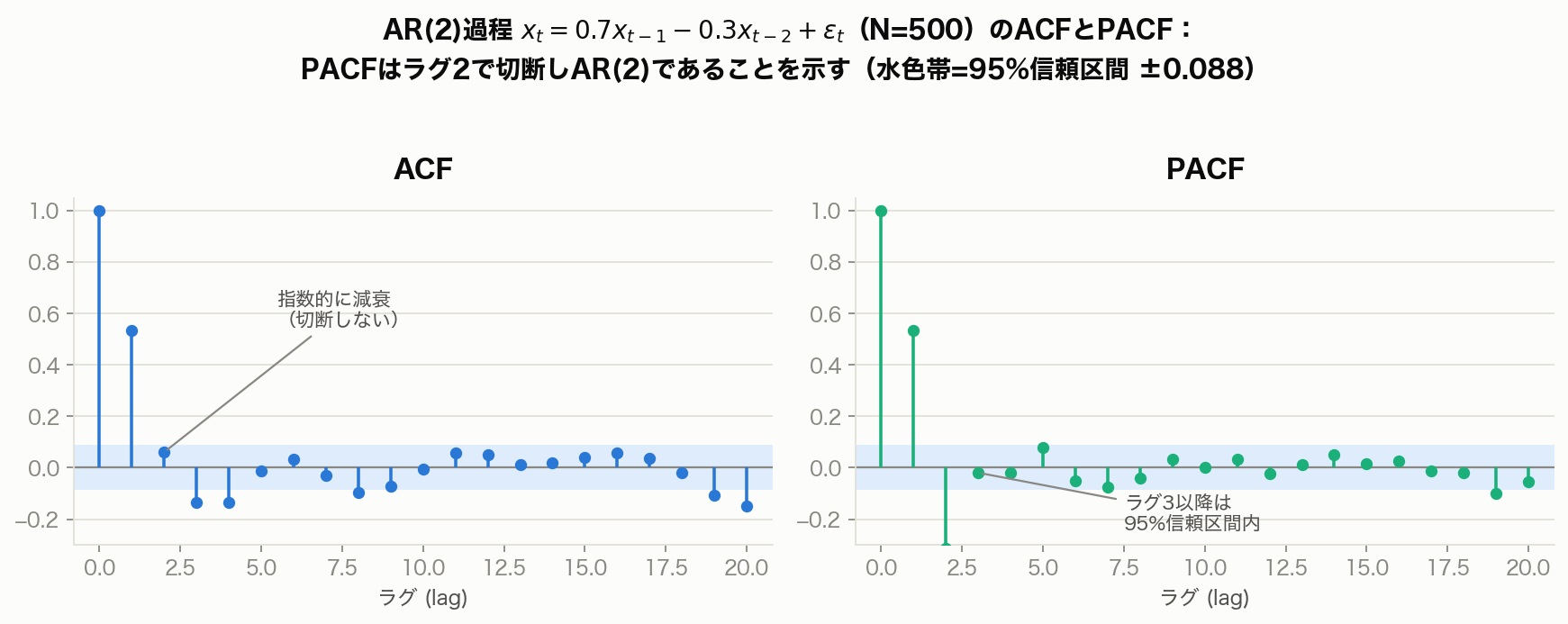
Extending the plot to nlags=20, only the PACF at lag 19 happens to poke outside the confidence band (a live example of the “roughly 5% by chance” caveat discussed later). The correct reading relies on the consecutive significance at low lags (1 and 2) to call the cutoff at lag 2, while ignoring the isolated spike at a high, unrelated lag.
Checking the PACF and innovation variance via Levinson-Durbin
levinson_durbin returns the recursion’s by-products—the PACF and innovation variance at every order—in one call.
from statsmodels.tsa.stattools import levinson_durbin

sigma_v, arcoefs, pacf_ld, sigma, _ = levinson_durbin(x, nlags=5, isacov=False)
print("PACF (Levinson-Durbin):", np.round(pacf_ld[1:6], 3))
print("innovation variance:", np.round(sigma[1:6], 3))
Output:
PACF (Levinson-Durbin): [ 0.532 -0.311 -0.02  -0.02   0.078]
innovation variance: [1.067 0.964 0.963 0.963 0.957]
The values differ from pacf(method="ywadjusted") only in the third decimal, because the underlying ACF estimator differs (with or without the small-sample bias adjustment). As equation \((10)\)
predicts, the innovation variance drops sharply from order 1 to order 2 (\(1.067 \to 0.964\)
) and then flattens out from order 3 onward (\(0.963, 0.963, 0.957\)
). The residual-variance side of the story says the same thing: raising the order beyond 2 does not improve prediction.
Order selection by AIC/BIC (AutoReg / ar_select_order)
We fit AR models of orders \(p = 0, \ldots, 6\)
to the same sample (using hold_back=10 to exclude the first 10 points and equalize the estimation sample) and compare AIC/BIC.
from statsmodels.tsa.ar_model import AutoReg, ar_select_order

print(f"{'p':>2} {'AIC':>9} {'BIC':>9}")
for p in range(0, 7):
    res = AutoReg(x, lags=p, hold_back=10, old_names=False).fit()
    print(f"{p:>2} {res.aic:>9.2f} {res.bic:>9.2f}")

sel_aic = ar_select_order(x, maxlag=10, ic="aic", old_names=False)
sel_bic = ar_select_order(x, maxlag=10, ic="bic", old_names=False)
print("lags selected by AIC:", sel_aic.ar_lags)
print("lags selected by BIC:", sel_bic.ar_lags)

res2 = AutoReg(x, lags=2, old_names=False).fit()
print("AutoReg(2) params:", np.round(res2.params, 3))
Output:
 p       AIC       BIC
 0   1592.91   1601.30
 1   1430.99   1443.57
 2   1381.90   1398.68
 3   1383.54   1404.51
 4   1385.38   1410.55
 5   1384.62   1413.98
 6   1385.15   1418.71
lags selected by AIC: [1, 2]
lags selected by BIC: [1, 2]
AutoReg(2) params: [ 0.006  0.702 -0.313]
Both AIC and BIC attain their minima at \(p = 2\)
(AIC \(= 1381.90\)
, BIC \(= 1398.68\)
), and ar_select_order picks lags \(\{1, 2\}\)
under either criterion. The PACF cutoff (lag 2) and the information-criterion choice (\(p = 2\)
) agree. The estimated coefficients \((\hat{\phi}_1, \hat{\phi}_2) = (0.702, -0.313)\)
also recover the true values \((0.7, -0.3)\)
accurately.
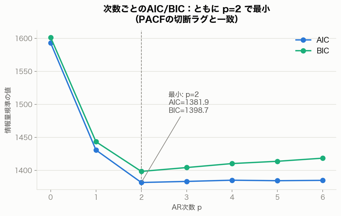
AIC and BIC both drop sharply from \(p=0\) to \(p=1\) (\(1592.91 \to 1430.99\) and \(1601.30 \to 1443.57\) ), fall further at \(p=2\) , then turn to a gentle increase from \(p=3\) onward. This “sharp drop, minimum, gentle rise” shape is itself the visual evidence for order identification—the PACF’s “cutoff” and the information criterion’s “minimum point” are the same phenomenon viewed from two different angles.
Searching over full ARMA orders (arma_order_select_ic / ARIMA)
Does AR(2) still win when MA terms are allowed as candidates? We check with arma_order_select_ic and fit the final model by maximum likelihood with ARIMA.
from statsmodels.tsa.stattools import arma_order_select_ic
from statsmodels.tsa.arima.model import ARIMA

order_sel = arma_order_select_ic(x, max_ar=4, max_ma=2, ic=["aic", "bic"])
print("AIC-minimizing order (p, q):", tuple(map(int, order_sel.aic_min_order)))
print("BIC-minimizing order (p, q):", tuple(map(int, order_sel.bic_min_order)))

arima_res = ARIMA(x, order=(2, 0, 0)).fit()
print("ARIMA(2,0,0) AR coefficients:", np.round(arima_res.arparams, 3))
print("ARIMA(2,0,0) residual variance:", round(arima_res.params[-1], 3))
Output:
AIC-minimizing order (p, q): (2, 0)
BIC-minimizing order (p, q): (2, 0)
ARIMA(2,0,0) AR coefficients: [ 0.7   -0.312]
ARIMA(2,0,0) residual variance: 0.96
Even searching the 2-D grid of \((p, q)\) (\(5 \times 3 = 15\) models), both AIC and BIC select \((2, 0)\) . The maximum-likelihood AR coefficients \((0.700, -0.312)\) and residual variance \(0.96\) (true value \(1.0\) ) are consistent as well. Three independent lines of evidence—PACF, AIC, and BIC—all point to AR(2), which is the ideal outcome of order identification.
Contrast experiments: an MA(2) process and white noise
Let us verify the remaining rows of the decision table numerically. We generate an MA(2) process \(x_t = \varepsilon_t + 0.6\varepsilon_{t-1} + 0.4\varepsilon_{t-2}\) and pure white noise, and run the same analysis.
# MA(2): the ACF should cut off after lag 2
np.random.seed(29)
theta = np.array([0.6, 0.4])
y = ArmaProcess(np.r_[1], np.r_[1, theta]).generate_sample(nsample=N)
acf_y = acf(y, nlags=10, fft=True)
pacf_y = pacf(y, nlags=10, method="ywadjusted")
print("MA(2) ACF  1-5:", np.round(acf_y[1:6], 3))
print("MA(2) PACF 1-5:", np.round(pacf_y[1:6], 3))
print("MA(2) significant ACF lags:",
      (np.where(np.abs(acf_y[1:]) > ci)[0] + 1).tolist())

# white noise: neither should be significant at any lag
np.random.seed(2)
w = np.random.randn(N)
acf_w = acf(w, nlags=10, fft=True)
pacf_w = pacf(w, nlags=10, method="ywadjusted")
print("WN ACF  1-5:", np.round(acf_w[1:6], 3))
print("WN PACF 1-5:", np.round(pacf_w[1:6], 3))
print("WN significant lags (ACF/PACF):",
      (np.where(np.abs(acf_w[1:]) > ci)[0] + 1).tolist(),
      (np.where(np.abs(pacf_w[1:]) > ci)[0] + 1).tolist())
Output:
MA(2) ACF  1-5: [ 0.598  0.31   0.065  0.003 -0.01 ]
MA(2) PACF 1-5: [ 0.599 -0.074 -0.142  0.065  0.009]
MA(2) significant ACF lags: [1, 2]
WN ACF  1-5: [-0.034  0.002  0.039 -0.027  0.039]
WN PACF 1-5: [-0.034  0.001  0.04  -0.025  0.038]
WN significant lags (ACF/PACF): [] []
A perfect mirror image of the AR(2) case. For the MA(2), the ACF cuts off after lag 2 (significant lags are exactly \(\{1, 2\}\) ; \(\hat{\rho}_3 = 0.065\) onward stays inside the band), while the PACF decays without cutting off: \(0.599 \to -0.074 \to -0.142\) . The sample values \(0.598\) and \(0.310\) are also reasonable against the theoretical \(\rho_1 = 0.553\) and \(\rho_2 = 0.263\) . For white noise, both ACF and PACF stay inside the confidence band at every lag—there is no structure to model.
Edge case: Yule-Walker bias near a unit root
All the experiments so far used a moderate sample of \(N=500\) . But when the true coefficient is close to a unit root (\(\phi \to 1\) ) and the sample is small, the Yule-Walker estimator—the PACF value itself—carries a non-negligible downward bias. We check this with a Monte Carlo experiment (5,000 replications each) on an AR(1) process with \(\phi = 0.95\) , tracking \(\hat{\alpha}(1)\) (the lag-1 PACF, i.e. the Yule-Walker estimate of \(\hat{\phi}_1\) ) as the sample size \(N\) varies.
import numpy as np
from statsmodels.tsa.arima_process import ArmaProcess
from statsmodels.tsa.stattools import pacf

np.random.seed(123)
phi_true = 0.95
reps = 5000
for n in [30, 100, 500, 2000]:
    estimates = np.zeros(reps)
    for i in range(reps):
        sample = ArmaProcess(np.r_[1, -phi_true], np.r_[1]).generate_sample(nsample=n)
        estimates[i] = pacf(sample, nlags=1, method="ywadjusted")[1]
    print(f"N={n:5d}  mean={estimates.mean():.4f}  "
          f"bias={estimates.mean() - phi_true:+.4f}  std={estimates.std():.4f}")
Output:
N=   30  mean=0.7658  bias=-0.1842  std=0.1327
N=  100  mean=0.8995  bias=-0.0505  std=0.0524
N=  500  mean=0.9420  bias=-0.0080  std=0.0160
N= 2000  mean=0.9480  bias=-0.0020  std=0.0073
Against the true value \(\phi = 0.95\) , at \(N=30\) the estimator averages \(0.766\) —a bias of \(-0.184\) (roughly a fifth of the true value)—with a large standard deviation of \(0.133\) . The bias shrinks roughly in proportion to \(1/N\) (\(-0.051\) at \(N=100\) , \(-0.008\) at \(N=500\) , \(-0.002\) at \(N=2000\) ), consistent with the Yule-Walker estimator’s known bias (on the order of \(-(1+3\phi)/N\) ). When a near-unit-root process is judged from a short sample, the cutoff-lag verdict itself tends to hold, but the point estimate of the coefficient can be substantially downward-biased. In practice, if a near-unit-root process is suspected, first check for a unit root with a test such as ADF, and consider bias-corrected estimation (e.g. bootstrap or bias-corrected Yule-Walker) rather than trusting the raw estimate.
Practical Caveats
- Stationarity is a prerequisite: both the PACF and Yule-Walker assume a stationary process. For series with trends or unit roots, first difference the data within the ARIMA framework (choose \(d\) ), then identify \(p\) and \(q\)
- The cutoff is a statistical cutoff: about 5% of lags will be significant by chance. Indeed, in our AR(2) experiment, extending the plot to lag 20 shows lag 19 spuriously crossing the band. Weight consecutive significance starting from low lags, and ignore isolated spikes at high lags
- Mixed ARMA cannot be settled by the table alone: when both ACF and PACF tail off, use the plots only to narrow candidates and delegate the decision to an information-criterion grid search such as
arma_order_select_ic - Do not skip residual diagnostics after identification: confirming that the chosen model’s residuals are white noise (residual ACF insignificant at all lags, Ljung-Box test not rejected) completes the workflow. Detecting leftover structure in residuals is the same idea as the residual analysis in time-series anomaly detection
- Near a unit root or with a small sample, the PACF point estimate carries a downward bias: as the Monte Carlo experiment above shows (bias \(-0.184\) for \(\phi=0.95\) , \(N=30\) ). The cutoff-lag verdict is robust, but discount the coefficient value accordingly
- The reflection coefficient can numerically fall outside the theoretical range \([-1, 1]\) : if the sample Toeplitz matrix built from the sample autocorrelations is not positive semi-definite (outlier contamination, imputed missing values, an extremely short series), the Levinson-Durbin recursion’s \(|\hat{\phi}_{kk}|\) can exceed 1, with the residual variance in equation \((10)\) going negative—a numerical breakdown that signals a departure from the stationarity assumption and a cue to revisit data preprocessing (outlier handling, imputation method)
- The PACF’s asymptotic theory can fail for non-Gaussian or count time series: the confidence band \(\pm 1.96/\sqrt{N}\) used in this article (equation \((11)\) ) is an asymptotic approximation that presumes a Gaussian linear process. Weiß et al. (2023) show that for integer-valued autoregressive (INAR-type) count time series, the conditions underlying this asymptotic approximation generally fail to hold, degrading the PACF test’s performance, and propose bootstrap-based alternatives. Apply the ACF/PACF decision table with caution to count data such as sales counts or incident counts
- Limits of linear models: the PACF captures linear dependence only. When nonlinear dependence dominates, a nonlinear model such as an LSTM becomes necessary. Even then, ACF/PACF remain useful for designing lag features and choosing input window lengths, sitting at the entrance of the pipeline organized in the machine learning for time series guide
Summary
- The partial autocorrelation (PACF) is the correlation after removing the linear effect of intermediate lags, and equals the last coefficient \(\phi_{kk}\) of an AR(k) regression
- Solving the Yule-Walker equations (a Toeplitz system) at increasing orders yields the PACF; the Levinson-Durbin recursion delivers coefficients, PACF, and innovation variances for all orders at once in \(O(p^2)\)
- Decision table for order identification: the PACF of AR(p) cuts off after lag \(p\) ; the ACF of MA(q) cuts off after lag \(q\) ; both tail off for ARMA
- In the AR(2) experiment, the PACF cutoff (\(\hat{\alpha}(2) = -0.312\)
significant, \(\hat{\alpha}(3)\)
onward within \(\pm 0.088\)
),
ar_select_orderunder AIC/BIC (both \(p = 2\) ), andarma_order_select_ic(both criteria at \((2, 0)\) ) all agreed - For MA(2) the ACF cut off instead (significant lags \(\{1, 2\}\) only), and for white noise neither function was significant at any lag—every row of the decision table was verified numerically
- The decision table and information criteria are complements, not competitors: narrow candidates visually, decide objectively with AIC/BIC, and close with a whiteness test of the residuals
- The Levinson-Durbin recursion can be derived from the projections of forward and backward prediction errors: the fact that the reflection coefficient equals the PACF (equation \((8d)\) ) and the fact that the PACF vanishes exactly beyond order \(p\) (the proof using equation \((10)\) ) are both consequences of the same projection argument
- As edge cases, we confirmed the downward bias of the Yule-Walker estimator near a unit root with a small sample (\(\phi=0.95\) , \(N=30\) gives bias \(-0.184\) ), the pathology of a reflection coefficient falling numerically outside \([-1,1]\) , and the breakdown of the PACF’s asymptotic theory for non-Gaussian, count time series (Weiß et al., 2023)
Related Articles
- Autocorrelation and Cross-Correlation: Theory and Python Implementation - The basics companion to this article, covering the ACF definition, fast FFT-based computation, and periodicity detection
- ARIMA and SARIMA Theory and Python Implementation - The practical follow-up that uses the orders \((p, d, q)\) identified here for actual forecasting
- ARMA/ARIMA in State-Space Form: Kalman-Filter Maximum Likelihood Estimation - Builds the state-space model using the order identified here and derives exact maximum likelihood estimation via the Kalman filter
- LSTM for Time Series Forecasting - A deep-learning approach for the nonlinear dependence the PACF cannot capture
- Time-Series Anomaly Detection - Residual-based anomaly detection methods sharing the whiteness-checking mindset of model diagnostics
- Machine Learning Hub for Time Series - A bird’s-eye view from classical ACF/PACF identification to state-space models and deep learning
References
- Box, G. E. P., Jenkins, G. M., Reinsel, G. C., & Ljung, G. M. (2015). Time Series Analysis: Forecasting and Control (5th ed.). Wiley.
- Brockwell, P. J., & Davis, R. A. (2016). Introduction to Time Series and Forecasting (3rd ed.). Springer.
- Durbin, J. (1960). “The fitting of time-series models.” Revue de l’Institut International de Statistique, 28(3), 233-244.
- Akaike, H. (1974). “A new look at the statistical model identification.” IEEE Transactions on Automatic Control, 19(6), 716-723.
- Weiß, C. H., Aleksandrov, B., Faymonville, M., & Jentsch, C. (2023). “Partial Autocorrelation Diagnostics for Count Time Series.” Entropy, 25(1), 105. https://doi.org/10.3390/e25010105
- statsmodels: statsmodels.tsa.stattools.pacf
- statsmodels: statsmodels.tsa.ar_model.AutoReg