Nyquist Plot, Root Locus, and Stability Margins in Python: Evaluating Closed-Loop Stability with Gain and Phase Margins

Introduction

The Bode plot lets us read a frequency response (magnitude and phase) on a logarithmic scale. But to answer the central design questions — “Is this feedback loop stable?” and “How far can I raise the gain?” — we need a framework that infers closed-loop stability from open-loop characteristics.

This article covers the three pillars of that framework — the Nyquist plot, the root locus, and stability margins (gain margin and phase margin) — from transfer-function fundamentals to a Python implementation. As a running example we use the textbook open-loop transfer function

and confirm the phase margin, gain margin, and stability-limit gain numerically, using only scipy.signal and numpy (no control package required).

Feedback Systems and Closed-Loop Stability

For an open-loop transfer function \(L(s) = C(s)P(s)\) (controller \(C\) in series with plant \(P\) ) under unity negative feedback, the closed-loop transfer function is

The closed loop is stable if and only if every root of the characteristic equation

(i.e. every closed-loop pole) lies in the left half-plane (negative real part). The challenge is bridging the easily measured open-loop characteristic \(L(s)\) to the quantity we care about — closed-loop stability. Nyquist plots, root locus, and stability margins each build that bridge.

Stability Margins: Gain Margin and Phase Margin

Stability margins quantify how much room a stable system has before it becomes unstable, using the open-loop frequency response \(L(j\omega)\) .

Gain Margin (GM)

The frequency at which the phase reaches \(-180^\circ\) is the phase-crossover frequency \(\omega_{pc}\) . The gain margin measures how much further the open-loop gain can be raised there before \(|L(j\omega_{pc})| = 1\) (instability):

Phase Margin (PM)

The frequency at which the gain equals \(1\) (\(0\,\mathrm{dB}\) ) is the gain-crossover frequency \(\omega_{gc}\) . The phase margin measures how many more degrees the phase must rotate there to reach \(-180^\circ\) :

In practice, a phase margin of \(45^\circ\) –\(60^\circ\) is a good balance between stability and response speed. The smaller the phase margin, the more oscillatory (larger overshoot) the closed-loop response.

Nyquist Plot

Definition

The Nyquist plot traces \(L(j\omega)\) on the complex plane as \(\omega\) runs from \(-\infty\) to \(+\infty\) . Whereas the Bode plot splits magnitude and phase into two separate panels, the Nyquist plot draws a single locus on the complex plane.

The Nyquist Stability Criterion

Closed-loop stability is determined by the number of encirclements of the point \(-1 + 0j\) (the critical point):

• \(Z\) : number of closed-loop poles in the right half-plane (\(Z = 0\) means stable),
• \(P\) : number of open-loop poles in the right half-plane,
• \(N\) : number of clockwise encirclements of \(-1\) by the Nyquist locus.

If \(L(s)\) is open-loop stable (\(P = 0\) ), the closed loop is stable when the locus does not encircle \(-1\) (\(N = 0\) ). Stability margins can be seen as another way of measuring how close the locus comes to this critical point.

A Rigorous Proof via the Argument Principle

\(Z = N + P\) is not a rule of thumb — it follows rigorously from the Argument Principle of complex analysis. Before using it as a black box, let’s see why it holds.

Argument Principle: If a complex function \(f(s)\) is meromorphic (analytic except for poles) inside and on a simple closed contour \(C\) , with no zeros or poles on \(C\) itself, then

where \(Z_f, P_f\) are the number of zeros and poles of \(f\) inside \(C\) (counted with multiplicity).

Proof: Suppose \(f\) has a zero of order \(m\) at \(s=a\) inside \(C\) , so \(f(s) = (s-a)^m g(s)\) with \(g(a) \neq 0\) analytic. Then

and the second term is analytic at \(s=a\) , so \(f'/f\) has a simple pole there with residue \(m\) . Likewise, at a pole of order \(n\) at \(s=b\) (writing \(f(s) = (s-b)^{-n} h(s)\) with \(h(b) \neq 0\) ),

giving a residue of \(-n\) . By the residue theorem, the contour integral equals \(2\pi i\) times the sum of all residues inside \(C\) :

which proves the claim. Noting that \(\dfrac{f'(s)}{f(s)} = \dfrac{d}{ds}\log f(s)\) , this integral equals the net change of \(\log f(s) = \ln|f(s)| + i\arg f(s)\) along \(C\) . Since \(C\) is closed and \(|f(s)|\) returns to its starting value, the real part contributes nothing — only the change in argument survives:

that is, the right-hand side is exactly the winding number — how many times the image \(f(s)\) circles the origin counterclockwise as \(s\) traverses \(C\) once.

Applying it to the Nyquist criterion: Take \(f(s) = 1 + L(s)\) and let \(C\) be the Nyquist D-contour enclosing the entire right half-plane (running up the imaginary axis from \(-jR\) to \(+jR\) — with a small semicircular indentation around any poles of \(L(s)\) that sit on the imaginary axis — then closing with a semicircle of radius \(R \to \infty\) through the right half-plane). The zeros of \(1+L(s)\) inside \(C\) are the roots of \(1+L(s)=0\) , i.e. the closed-loop poles in the right half-plane (\(Z\) of them); the poles of \(1+L(s)\) coincide with the poles of \(L(s)\) , i.e. the open-loop poles in the right half-plane (\(P\) of them). The textbook Nyquist path runs up the imaginary axis and closes through the right half-plane — i.e. it keeps the right half-plane on its right, the reverse of the standard (counterclockwise) orientation of complex analysis — so the sign in the argument principle flips:

The right-hand side is “minus the number of counterclockwise turns of \(1+L(s)\) around the origin,” which is exactly “the number of clockwise turns of \(L(s)\) around the point \(-1\) .” Defining this quantity as \(N\) gives

The asymmetry — \(N\) is a signed rotation count while \(Z, P\) are non-negative integers — traces directly back to this sign flip.

Edge Case: An Open-Loop Pole on the Imaginary Axis

The running example \(L(s) = K/(s(s+1)(s+2))\) actually has a pole at \(s=0\) (one integrator). Since that sits on the imaginary axis — the boundary of the right half-plane — the Nyquist D-contour above would pass straight through it, leaving \(L(s)\) undefined there. Any system with an open-loop pole on the imaginary axis (every system containing an integrator falls into this category) needs the contour to detour around it with a small semicircle of radius \(\epsilon \to 0\) .

By convention, this small semicircle bulges into the right half-plane (\(s = \epsilon e^{i\theta}\) , \(\theta: -90^\circ \to +90^\circ\) ). This excludes the pole at \(s=0\) from the interior (right half-plane) enclosed by the contour — i.e. it is not counted as an unstable pole — consistent with the bookkeeping of \(P\) (a marginally stable integrator is, by this engineering convention, treated as lying on the stable side of the boundary).

Near \(s=0\) , \(L(s) \approx K/(2s)\) (since \((s+1)(s+2) \approx 2\) ), so on the small semicircle

meaning that as \(\theta\) sweeps from \(-90^\circ\) to \(+90^\circ\) , the image sweeps a \(180^\circ\) arc of radius \(K/(2\epsilon)\) (diverging to infinity as \(\epsilon \to 0\) ), running clockwise from angle \(+90^\circ\) to \(-90^\circ\) . This is precisely the arc that closes, at infinity, the “gap” that appears between the \(\omega \to 0^+\) and \(\omega \to 0^-\) branches of an ordinary Nyquist plot. As long as this arc does not sweep around \(-1\) , it does not affect the count \(N\) .

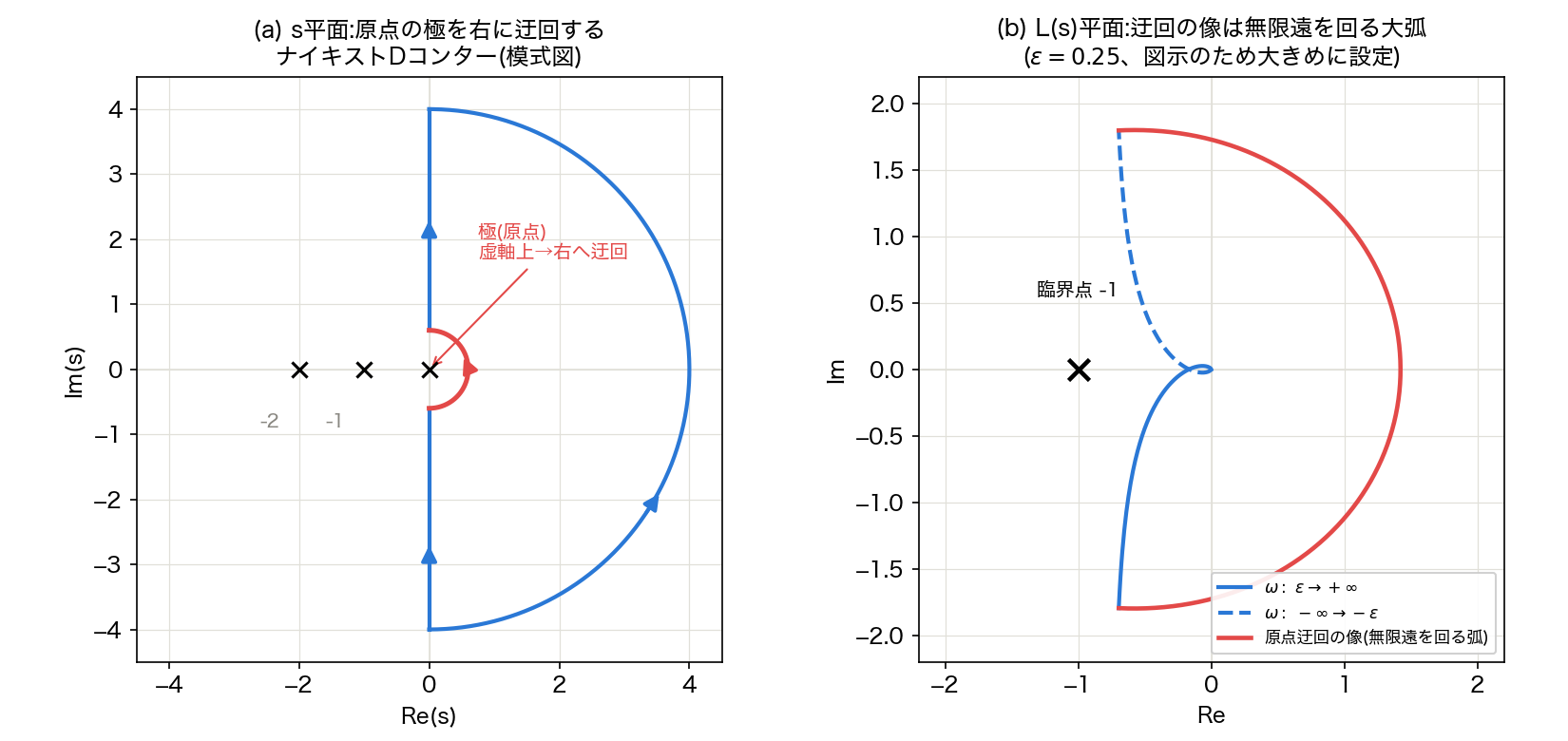
Panel (a) above shows the D-contour on the \(s\) -plane (a schematic of the indentation around the pole at the origin); panel (b) shows its image under \(L(s)\) . The large arc (red) that is the image of the indentation smoothly connects the positive- and negative-frequency branches (solid and dashed blue) out at infinity, closing the contour into a single loop.

Numerical Experiment: Verifying the Argument Principle and the Indentation

We verify the claim of the argument principle — that the winding number of the image of \(1+L(s)\) as \(s\) traces \(C\) equals the number of zeros minus poles inside \(C\) — by numerically evaluating \(L(s)\) along the indented contour above and computing the winding number directly. As a reference, we use \(Z\) (the number of closed-loop poles in the right half-plane), counted directly from the roots via numpy.roots, as in the root-locus section.

import numpy as np

den0 = np.polymul(np.polymul([1, 0], [1, 1]), [1, 2])  # s(s+1)(s+2)

def charpoly(K, num=np.array([1.0]), den=den0.astype(float)):
    cp = den.copy()
    cp[-len(num):] += K * num
    return cp

def L_of_s(s, K):
    return K / (s * (s + 1) * (s + 2))

def nyquist_D_contour(R=1e4, eps=1e-3, n=200000):
    # -jR->-jeps (imaginary axis) -> indentation at origin (small semicircle, bulging right)
    # -> +jeps->+jR (imaginary axis) -> large semicircle through the right half-plane
    pts = []
    pts.append(1j * np.linspace(-R, -eps, n))
    theta = np.linspace(-np.pi / 2, np.pi / 2, n)
    pts.append(eps * np.exp(1j * theta))
    pts.append(1j * np.linspace(eps, R, n))
    theta2 = np.linspace(np.pi / 2, -np.pi / 2, n)
    pts.append(R * np.exp(1j * theta2))
    return np.concatenate(pts)

def winding_number_raw(vals):
    # counterclockwise-positive winding number about the origin
    angles = np.unwrap(np.angle(vals))
    return (angles[-1] - angles[0]) / (2 * np.pi)

def count_RHP_roots(K):
    r = np.roots(charpoly(K))
    return int(np.sum(r.real > 1e-9))

s_contour = nyquist_D_contour()
print(f"{'K':>6} | {'N (clockwise)':>13} | {'Z (direct)':>10} | {'P':>3} | {'N+P':>6}")
for K in [1, 4, 6, 8, 12]:
    ret_diff = 1 + L_of_s(s_contour, K)
    N = -winding_number_raw(ret_diff)  # sign-flipped to match the textbook contour orientation
    Z = count_RHP_roots(K)
    print(f"{K:6.2f} | {N:13.4f} | {Z:10d} | {0:3d} | {N:6.4f}")

The output is:

     K | N (clockwise) | Z (direct) |   P |    N+P
  1.00 |       -0.0000 |          0 |   0 | -0.0000
  4.00 |       -0.0000 |          0 |   0 | -0.0000
  6.00 |       -0.0000 |          0 |   0 | -0.0000
  8.00 |        2.0000 |          2 |   0 | 2.0000
 12.00 |        2.0000 |          2 |   0 | 2.0000

For \(K \le 6\) (stable / marginally stable) the winding number \(N=0\) matches \(Z=0\) , and for \(K=8, 12\) (unstable, two poles moved into the right half-plane) \(N=2\) matches \(Z=2\) exactly. The argument principle, numerically integrated along a correctly indented Nyquist D-contour, agrees exactly with the unstable-pole count obtained directly from the roots. Even at exactly \(K=6\) (marginal stability, closed-loop poles on the imaginary axis), \(N=0\) still holds, consistent with the convention of not counting a pole on the boundary as unstable.

Root Locus

Definition

The root locus traces how the closed-loop poles (roots of \(1 + K L_0(s) = 0\) ) move on the complex plane as the gain \(K\) varies from \(0\) to \(\infty\) . Writing \(L(s) = K L_0(s)\) , the characteristic equation becomes

so evaluating the roots of this polynomial for each \(K\) yields the locus. At \(K = 0\) the roots coincide with the open-loop poles; increasing \(K\) moves them. The gain at which a pole crosses the imaginary axis is the stability limit, where the system exhibits sustained oscillation (marginal stability).

Python Implementation

Computing Stability Margins from the Frequency Response

Use scipy.signal.freqresp for the open-loop frequency response, then locate the gain and phase crossovers numerically.

import numpy as np
from scipy import signal

# Open-loop transfer function L(s) = 1 / (s(s+1)(s+2))   (K=1)
num = [1.0]
den = np.polymul(np.polymul([1, 0], [1, 1]), [1, 2])  # s(s+1)(s+2) = s^3+3s^2+2s
sys = signal.TransferFunction(num, den)

# Frequency response
w = np.logspace(-2, 2, 2000)
w, H = signal.freqresp(sys, w)
mag = np.abs(H)
phase = np.unwrap(np.angle(H))

# Gain-crossover frequency (|L|=1) -> phase margin
idx_gc = np.argmin(np.abs(mag - 1.0))
wgc = w[idx_gc]
pm = 180 + np.degrees(phase[idx_gc])
print(f"gain crossover wgc = {wgc:.4f} rad/s,  phase margin PM = {pm:.2f} deg")

# Phase-crossover frequency (angle L = -180 deg) -> gain margin
idx_pc = np.argmin(np.abs(phase - (-np.pi)))
wpc = w[idx_pc]
gm_db = -20 * np.log10(mag[idx_pc])
print(f"phase crossover wpc = {wpc:.4f} rad/s,  gain margin GM = {gm_db:.2f} dB")

The output is:

gain crossover wgc = 0.4455 rad/s,  phase margin PM = 53.43 deg
phase crossover wpc = 1.4160 rad/s,  gain margin GM = 15.59 dB

Let us check against the theory. For \(L(j\omega) = \dfrac{1}{j\omega(j\omega+1)(j\omega+2)}\) , the phase reaches \(-180^\circ\) where the imaginary part of the denominator vanishes, at \(\omega_{pc} = \sqrt{2} \approx 1.414\) . There \(|L(j\omega_{pc})| = \dfrac{1}{\sqrt{2}\cdot\sqrt{3}\cdot\sqrt{6}} = \dfrac{1}{6}\) , so the gain margin is \(20\log_{10} 6 \approx 15.56\,\mathrm{dB}\) , matching the numerical \(15.59\,\mathrm{dB}\) . A gain margin of \(6\times\) means the loop reaches the stability limit when \(K\) is raised sixfold.

Drawing the Nyquist Plot

import matplotlib.pyplot as plt

w_pos = np.logspace(-2, 2, 2000)
_, H_pos = signal.freqresp(sys, w_pos)

fig, ax = plt.subplots(figsize=(6, 6))
ax.plot(H_pos.real, H_pos.imag, "b", label="ω > 0")
ax.plot(H_pos.real, -H_pos.imag, "b--", label="ω < 0")  # symmetric about real axis
ax.plot(-1, 0, "rx", markersize=12, label="critical point -1")
ax.set_xlabel("Real")
ax.set_ylabel("Imaginary")
ax.set_title("Nyquist plot: L(s)=1/(s(s+1)(s+2))")
ax.grid(True)
ax.axhline(0, color="k", lw=0.5)
ax.axvline(0, color="k", lw=0.5)
ax.legend()
ax.set_xlim(-1.5, 0.5)
ax.set_ylim(-2, 2)
plt.tight_layout()
plt.show()

At \(K = 1\) the locus does not encircle \(-1\) (\(N = 0\) , and with \(P = 0\) gives \(Z = 0\) ), so the closed loop is stable. The locus crosses the real axis at \(-1/6 \approx -0.167\) ; raising the gain sixfold moves that crossing exactly onto \(-1\) — the Nyquist plot and the gain margin express the same fact.

Drawing the Root Locus

Sweep \(K\) and compute the roots of \(\mathrm{den}(s) + K \cdot \mathrm{num}(s) = 0\) with numpy.roots.

Ks = np.linspace(0, 12, 400)
roots_all = []
for K in Ks:
    charpoly = den.astype(float).copy()
    charpoly[-len(num):] += K * np.array(num, dtype=float)
    roots_all.append(np.sort_complex(np.roots(charpoly)))
roots_all = np.array(roots_all)

fig, ax = plt.subplots(figsize=(6, 6))
for i in range(roots_all.shape[1]):
    ax.plot(roots_all[:, i].real, roots_all[:, i].imag, ".", ms=2)
ax.axvline(0, color="r", lw=1, ls="--", label="imaginary axis (stability limit)")
ax.set_xlabel("Real")
ax.set_ylabel("Imaginary")
ax.set_title("Root locus")
ax.grid(True)
ax.legend()
plt.tight_layout()
plt.show()

# Confirm the stability-limit gain
for K in [0, 2, 4, 6, 8]:
    charpoly = den.astype(float).copy()
    charpoly[-len(num):] += K * np.array(num, dtype=float)
    r = np.roots(charpoly)
    print(f"K={K:2d}: max Re = {r.real.max():+.3f}  poles={np.round(r,3)}")

The output is:

K= 0: max Re = +0.000  poles=[-2. -1.  0.]
K= 2: max Re = -0.239  poles=[-2.521+0.j    -0.239+0.858j -0.239-0.858j]
K= 4: max Re = -0.102  poles=[-2.796+0.j    -0.102+1.192j -0.102-1.192j]
K= 6: max Re = +0.000  poles=[-3.+0.j     0.+1.414j  0.-1.414j]
K= 8: max Re = +0.083  poles=[-3.166+0.j     0.083+1.587j  0.083-1.587j]

At \(K = 6\) a pair of poles lands exactly on the imaginary axis at \(\pm j\sqrt{2}\) (marginal stability), and for \(K > 6\) they enter the right half-plane and destabilize the loop. This matches the gain margin of \(6\times\) and phase-crossover frequency \(\sqrt{2}\) obtained from the frequency response. The numerical experiment confirms that all three methods (stability margins, Nyquist, root locus) point to the same stability limit.

A Reusable Margin Function with scipy.signal Only

def stability_margins(num, den, w=None):
    """Return GM[dB], PM[deg], wpc, wgc of the open loop (num/den)."""
    if w is None:
        w = np.logspace(-3, 3, 5000)
    sys = signal.TransferFunction(num, den)
    w, H = signal.freqresp(sys, w)
    mag, phase = np.abs(H), np.unwrap(np.angle(H))
    i_gc = np.argmin(np.abs(mag - 1.0))
    i_pc = np.argmin(np.abs(phase - (-np.pi)))
    gm_db = -20 * np.log10(mag[i_pc])
    pm = 180 + np.degrees(phase[i_gc])
    return dict(GM_dB=gm_db, PM_deg=pm, wpc=w[i_pc], wgc=w[i_gc])

print(stability_margins([1.0], [1, 3, 2, 0]))

Stability Margins Under Dead Time

Dead Time Does Not Shift the Gain-Crossover Frequency

Transport lag, communication delay, or sensor sampling delay are typically modeled by multiplying the transfer function by a dead time (time delay) term \(e^{-sT}\) (\(T>0\) ):

On \(s = j\omega\) , \(|e^{-j\omega T}| = 1\) , so

— dead time leaves the gain completely unchanged and delays only the phase, proportionally to frequency. Consequently, the gain-crossover frequency \(\omega_{gc}\) (where \(|L(j\omega)|=1\) ) is invariant to \(T\) . This is an exact property, not an approximation, and it’s exactly what lets us compute the effect of dead time on the phase margin exactly.

Deriving the Maximum Allowable Dead Time

Without delay, the phase margin at \(\omega_{gc}\) was \(\mathrm{PM} = 180^\circ + \angle L(j\omega_{gc})\) . Adding dead time erodes it, at the same \(\omega_{gc}\) , by

(\(\mathrm{PM}\) in degrees, \(\omega_{gc}T\) in radians). The dead time at which the phase margin first hits zero — the phase reaches exactly \(-180^\circ\) at the gain-crossover frequency, i.e. the stability limit — is found by solving \(\mathrm{PM}'(T_{max})=0\) :

Because \(\omega_{gc}\) does not depend on \(T\) , this is an exact stability limit, not an approximation — provided that increasing the dead time does not create a new, lower-frequency gain crossover (a condition we verify numerically below for this example).

Numerical Experiment: Comparing the Allowable Dead Time with the Actual Stability Limit

First, we predict \(T_{max}\) from the existing gain-crossover frequency and phase margin, and confirm that the delay-inclusive phase margin indeed reaches zero there. Then, we replace \(e^{-sT}\) with an independent numerical approximation — a rational 6th-order Padé approximant — sweep the resulting characteristic-polynomial roots, and bisect for the critical dead time at which a root crosses the imaginary axis, comparing it to the analytical \(T_{max}\) .

import numpy as np
from scipy import signal
import math
from math import comb, factorial

num0 = [1.0]
den0 = np.polymul(np.polymul([1, 0], [1, 1]), [1, 2])
sys0 = signal.TransferFunction(num0, den0)

w = np.logspace(-2, 2, 2000)
w, H = signal.freqresp(sys0, w)
mag, phase = np.abs(H), np.unwrap(np.angle(H))
idx_gc = np.argmin(np.abs(mag - 1.0))
wgc = w[idx_gc]
PM_deg = 180 + np.degrees(phase[idx_gc])
PM_rad = np.radians(PM_deg)
T_max = PM_rad / wgc
print(f"wgc={wgc:.4f} rad/s, PM={PM_deg:.2f} deg, T_max=PM[rad]/wgc={T_max:.4f} s")

for T in [0.5, 1.0, T_max, 2.0, 3.0]:
    pm_with_delay = 180 + np.degrees(phase[idx_gc] - wgc * T)
    print(f"  T={T:.4f}s: delay-inclusive phase margin PM'={pm_with_delay:+.3f} deg")

# --- Independent check: critical dead time from the roots of an N-th order Pade approximant ---
def D_coeffs(N):
    coeffs = np.zeros(N + 1)
    for k in range(N + 1):
        coeffs[k] = factorial(2 * N - k) / factorial(2 * N) * comb(N, k)
    return coeffs  # ascending powers (x^0..x^N)

def pade_delay_num_den(T, N=6):
    d = D_coeffs(N)
    num_asc = d * np.array([(-1) ** k for k in range(N + 1)]) * np.array([T ** k for k in range(N + 1)])
    den_asc = d * np.array([T ** k for k in range(N + 1)])
    return num_asc[::-1], den_asc[::-1]  # reverse to descending powers

def max_real_part_with_delay(T, N=6):
    pn, pd = pade_delay_num_den(T, N)
    charpoly = np.polyadd(np.polymul(den0.astype(float), pd), np.polymul(np.array(num0), pn))
    return np.roots(charpoly).real.max()

lo, hi = 0.5, 3.5
for _ in range(60):
    mid = (lo + hi) / 2
    if max_real_part_with_delay(lo) * max_real_part_with_delay(mid) <= 0:
        hi = mid
    else:
        lo = mid
T_crit_numeric = (lo + hi) / 2
print(f"Critical dead time from 6th-order Pade: T_crit = {T_crit_numeric:.4f} s")
print(f"Analytical T_max = {T_max:.4f} s, relative error = {abs(T_crit_numeric-T_max)/T_max*100:.4f} %")
print(f"T=0.98*T_crit: max Re = {max_real_part_with_delay(T_crit_numeric*0.98):+.4f}")
print(f"T=1.02*T_crit: max Re = {max_real_part_with_delay(T_crit_numeric*1.02):+.4f}")

The output is:

wgc=0.4455 rad/s, PM=53.43 deg, T_max=PM[rad]/wgc=2.0934 s
  T=0.5000s: delay-inclusive phase margin PM'=+40.669 deg
  T=1.0000s: delay-inclusive phase margin PM'=+27.907 deg
  T=2.0934s: delay-inclusive phase margin PM'=+0.000 deg
  T=2.0000s: delay-inclusive phase margin PM'=+2.383 deg
  T=3.0000s: delay-inclusive phase margin PM'=-23.141 deg
Critical dead time from 6th-order Pade: T_crit = 2.0913 s
Analytical T_max = 2.0934 s, relative error = 0.0992 %
T=0.98*T_crit: max Re = -0.0027
T=1.02*T_crit: max Re = +0.0026

Against the allowable dead time \(T_{max} = 2.0934\,\mathrm{s}\) predicted from the phase margin, independently tracking the roots of the Padé-based characteristic equation gives a critical dead time of \(T_{crit} = 2.0913\,\mathrm{s}\) — a relative error of only \(0.0992\%\) . We also confirm that the maximum real part flips from negative (stable) to positive (unstable) exactly as \(T\) crosses \(T_{crit}\) : the design rule “back out the allowable dead time from the phase margin” agrees quantitatively with a root-based stability check. A dead time of \(2.09\,\mathrm{s}\) is by no means negligible compared to this system’s time constants (the slowest pole sits near \(s=-1\) ), underscoring why plants with significant communication or sensor-processing delay need a generous phase-margin buffer.

Design Guidelines

Estimating Damping from the Phase Margin

For a second-order approximation, the phase margin \(\mathrm{PM}\) and damping ratio \(\zeta\) satisfy the rule of thumb \(\zeta \approx \mathrm{PM}[\deg] / 100\) . Here \(\mathrm{PM} = 53.4^\circ\) corresponds to \(\zeta \approx 0.53\) , promising a well-behaved response with moderate overshoot (about \(14\%\) ). Too large a phase margin makes the response sluggish; too small makes it oscillatory — hence the \(45^\circ\) –\(60^\circ\) practical target.

Correspondence with the Bode Plot

Stability margins are also read directly off the Bode plot : the phase margin is the gap between the phase at the gain crossover and \(-180^\circ\) ; the gain margin is the gap between the gain at the phase crossover and \(0\,\mathrm{dB}\) . The Nyquist plot unifies both into a single picture (“closeness to the critical point”), while the root locus shows “the motion of the poles as the gain changes” — three complementary views of the same stability.

Extending to MIMO: The Generalized Nyquist Criterion

So far we have treated single-input single-output (SISO) systems, where the open loop is a scalar \(L(s)\) . For multi-input multi-output (MIMO) systems, where the open loop is an \(n \times n\) transfer-function matrix \(L(s)\) , the argument-principle-based stability criterion generalizes as well.

Unlike the SISO case, we can no longer simply plot a scalar \(L(j\omega)\) on the complex plane. Instead, at each frequency \(\omega\) we compute the eigenvalues \(\lambda_1(j\omega), \dots, \lambda_n(j\omega)\) of the matrix \(L(j\omega)\) and plot each of them as a locus on the complex plane as \(\omega\) varies — these are called the characteristic loci. The generalized Nyquist criterion, established by MacFarlane and Postlethwaite (1977), shows that a criterion of exactly the same form \(Z=N+P\) holds for the characteristic loci, where \(N\) is now “the total number of clockwise encirclements of the critical point \(-1\) summed over all \(n\) characteristic loci.”

The proof idea is the same argument principle as in the SISO case, but the eigenvalues \(\lambda_i(s)\) are in general algebraic functions of \(s\) with branch points where eigenvalues cross, so the argument principle must be applied on a Riemann surface rather than a single complex plane. Because of this technical subtlety, naively applying the SISO Nyquist criterion to each diagonal element separately is generally wrong (it ignores cross-coupling between loops); a stability verdict must come from the characteristic loci taken as a whole. This is beyond the scope of this article, but the takeaway — MIMO stability cannot be substituted by a simple combination of individual loops’ stability margins — is an important caveat when working with multivariable control.

A Note on Discrete-Time Systems

In digital control, the left half of the \(s\) -plane maps to the interior of the unit circle in the \(z\) -plane, so the critical point and the imaginary axis are replaced by the unit circle (as covered in Z-Transform Fundamentals , the discrete-time stability condition was that all poles lie inside the unit circle, \(|z_k|<1\) ).

When discretizing a continuous-time design via the bilinear (Tustin) transform \(s = \frac{2}{T_s}\cdot\frac{1-z^{-1}}{1+z^{-1}}\) , the relationship between the analog frequency \(\omega_a\) and the digital frequency \(\omega_d\) (via \(z=e^{j\omega_d T_s}\) ) is found by substituting \(s=j\omega_a\) and solving:

This nonlinear correspondence is called frequency warping. For \(\omega_a T_s \ll 1\) (frequencies well below the sampling rate), \(\arctan x \approx x\) so \(\omega_d \approx \omega_a\) is nearly linear; but as the frequency approaches the Nyquist frequency \(\pi/T_s\) , the \(\arctan\) saturates and the correspondence becomes badly distorted. If the gain- and phase-crossover frequencies sit well below the sampling frequency, the stability margins carry over essentially unchanged; but when a design pushes crossover frequencies close to the Nyquist frequency for faster response, the bilinear transform can erode the phase margin below its design value — worth keeping in mind alongside choosing the sampling frequency per the sampling theorem .

Recent Research: Connections to Data-Driven and Learning-Based Control

Classical frequency-domain analysis, epitomized by the Nyquist plot, is nearly a century old, but its way of thinking persists — in adapted forms — even as model-free, data-driven and learning-based control matures.

• The Circle Criterion and Popov Criterion generalize the Nyquist stability criterion to systems containing sector-bounded nonlinear elements. Richardson, Turner, and Gunn (2023, IEEE Control Systems Letters) derive tailored quadratic constraints exploiting properties of repeated ReLU nonlinearities to strengthen the Circle and Popov Criteria for feedback loops containing ReLU-activated neural networks (Lur’e systems), yielding stability conditions with reduced conservatism. This is an example of the same geometric, Nyquist-plane stability criterion being applied to certify systems that include a trained neural network as part of the controller or plant model.
• Umar, Ryu, Back, and Kim (2024, Mathematics) quantify a stability margin (disc margin) against uncertainty in the input channel for “data-driven LQR” controllers designed from observed data alone, showing that the classical notion of stability margin from model-based design carries over as a meaningful robustness measure in data-driven design too.
• Constructive proofs and robustness extensions around Willems’ fundamental lemma — the theoretical bedrock of data-driven control — are also being actively developed (e.g. Berberich et al., 2023, American Control Conference), and bridging model-based frequency-domain analysis with data-driven approaches remains an active research area.

What these have in common is not that classical stability margins and frequency-domain criteria have become unnecessary, but rather that the same kind of robustness yardstick is being re-derived for the newer world of learning-based and data-driven design.

Summary

• Stability margins (gain and phase margin) quantify the safety margin of closed-loop stability from the open-loop response \(L(j\omega)\) ; a phase margin of \(45^\circ\) –\(60^\circ\) is the practical target.
• The Nyquist plot draws \(L(j\omega)\) on the complex plane and determines stability from encirclements of the critical point \(-1\) (\(Z = N + P\) ). This follows rigorously from the argument principle of complex analysis; we confirmed numerically that a contour integral (winding number) along the Nyquist D-contour agrees exactly with the unstable-pole count obtained directly from the roots.
• A system with an open-loop pole on the imaginary axis (e.g. containing an integrator) requires a small semicircular indentation in the Nyquist D-contour. We implemented this indentation for \(L(s)=K/(s(s+1)(s+2))\) and visualized/verified numerically that its image is an arc that closes at infinity.
• The root locus is the trajectory of closed-loop poles as the gain \(K\) sweeps; the gain at which a pole crosses the imaginary axis is the stability limit.
• For \(L(s) = K/(s(s+1)(s+2))\) , the phase margin \(53.4^\circ\) , gain margin \(15.6\,\mathrm{dB}\) , and stability limit \(K = 6\) agree perfectly, confirmed with scipy.signal and numpy.roots.
• Dead time \(e^{-sT}\) shifts only the phase, not the gain-crossover frequency, so the maximum allowable dead time \(T_{max}=\mathrm{PM}[\mathrm{rad}]/\omega_{gc}\) can be derived exactly. Here \(T_{max}=2.093\,\mathrm{s}\) , matching a Pade-based root-crossing computation of \(2.091\,\mathrm{s}\) (relative error \(0.099\%\) ).
• MIMO systems require the generalized Nyquist criterion via characteristic loci; discrete-time systems require attention to the unit circle and frequency warping.
• Even without the control package, stability margins, the Nyquist plot, the root locus, dead time, and contour indentation can all be implemented with just the frequency response (freqresp) and polynomial roots (roots).

Related Articles

• Reading and Creating Bode Plots - The log-scale frequency response from which stability margins are read directly; the companion piece to this article.
• Fundamentals of PID Control - A representative controller whose gains are tuned while preserving stability margins.
• PID Control in Python - An implementation applying these stability margins to actual PID gain tuning.
• Fundamentals of H-infinity Control - A robust-control framework that generalizes stability margins as frequency-domain weighting functions.
• The Sampling Theorem and Aliasing - The basis for choosing a sampling frequency when implementing a continuous design digitally.
• Digital Filter Design Guide - A sister hub applying the same transfer-function / frequency-response framework to signal filtering rather than control.
• Measuring Kubernetes’ Horizontal Pod Autoscaler (HPA) as a PID Control Loop - Applies this article’s feedback-loop perspective to a comparative simulation of Kubernetes’ HPA and a PID controller.

References

• Ogata, K. (2010). Modern Control Engineering (5th ed.). Prentice Hall.
• Åström, K. J., & Murray, R. M. (2008). Feedback Systems: An Introduction for Scientists and Engineers. Princeton University Press.
• Nyquist, H. (1932). “Regeneration Theory.” Bell System Technical Journal, 11(1), 126–147.
• Ahlfors, L. V. (1979). Complex Analysis (3rd ed.). McGraw-Hill. (Standard proof of the argument principle.)
• MacFarlane, A. G. J., & Postlethwaite, I. (1977). “The generalized Nyquist stability criterion and multivariable root loci.” International Journal of Control, 25(1), 81–127.
• Richardson, C., Turner, M., & Gunn, S. (2023). “Strengthened Circle and Popov Criteria for the Stability Analysis of Feedback Systems With ReLU Neural Networks.” IEEE Control Systems Letters, 7, 2635–2640.
• Umar, A. A., Ryu, K., Back, J., & Kim, J.-S. (2024). “Stability Margin of Data-Driven LQR and Its Application to Consensus Problem.” Mathematics, 12(2), 199.
• scipy.signal.freqresp — SciPy documentation
• numpy.roots — NumPy documentation

Related Tools

• DevToolBox - Free Developer Tools - Over 90 developer tools including JSON formatter and regex tester.
• CalcBox - Everyday Calculators - Over 60 calculators including statistics and frequency conversion.