Two Problems EEMD Doesn’t Solve
https://yuhi-sa.github.io/en/posts/20260528_mode_decomposition/1/ covered the basics of EMD, VMD, and SSA, along with EMD’s mode mixing problem and EEMD (Ensemble EMD), which suppresses mode mixing by averaging over noise-perturbed trials. However, EEMD introduces two side effects of its own:
- Incomplete reconstruction: the noise added in each trial does not perfectly cancel out, so the sum of all IMFs does not exactly equal the original signal
- Mode splitting: a single physical component gets scattered across multiple adjacent IMFs (the opposite failure mode from mixing)
This article explains CEEMDAN (Complete Ensemble EMD with Adaptive Noise), which was proposed to fix both issues, from first principles. We implement it in Python (PyEMD) and compare it numerically against EMD and EEMD. We then implement the marginal Hilbert spectrum, the central tool for using the Hilbert-Huang Transform in practice, and the envelope spectrum method standard in bearing fault diagnosis, verified on a synthetic bearing-defect signal.
1. The CEEMDAN Algorithm
1.1 Why EEMD Fails to Reconstruct Exactly
EEMD adds \(I\) independent white-noise realizations \(n_i(t)\) to the signal \(x(t)\) , runs EMD on each \(x(t) + n_i(t)\) , and averages the resulting IMFs:
\[ \mathrm{IMF}_k^{\mathrm{EEMD}}(t) = \frac{1}{I} \sum_{i=1}^{I} \mathrm{IMF}_k^{(i)}(t) \]Because EMD is a nonlinear operation, it does not commute with averaging: “decompose the noisy signal and then average” is mathematically not the same as “decompose the original signal directly.” With a finite number of trials \(I\) , the sum of all averaged IMFs therefore does not exactly return \(x(t)\) .
1.2 CEEMDAN’s Stage-Wise Noise Removal
CEEMDAN (Torres et al., 2011) eliminates this error in principle by adding noise only to the current residual at each stage and extracting one true mode at a time.
Let \(r_{k-1}(t)\) be the residual after stage \(k-1\) (\(r_0 = x\) ), and let \(E_1[\cdot]\) denote “add white noise to a signal, run EMD, and return the first IMF.” Then:
\[ \begin{aligned} \mathrm{IMF}_1 &= \frac{1}{I} \sum_{i=1}^{I} E_1[x + \epsilon_0 n_i] \\ r_1 &= x - \mathrm{IMF}_1 \\ \mathrm{IMF}_k &= \frac{1}{I} \sum_{i=1}^{I} E_1[r_{k-1} + \epsilon_{k-1} E_{k-1}[n_i]] \\ r_k &= r_{k-1} - \mathrm{IMF}_k \end{aligned} \]The noise at each stage is the original white noise \(n_i\) passed through the EMD operators of the previous stages, so the added noise stays consistent with the decomposition. This construction guarantees:
\[ x(t) = \sum_{k=1}^{K} \mathrm{IMF}_k(t) + r_K(t) \]as an identity, regardless of the number of ensemble trials. CEEMDAN therefore keeps EEMD’s benefit (suppressing mode mixing) while recovering EMD’s original property of exact reconstruction.
1.3 Stopping Criteria and Practical Caveats
Four points matter when using CEEMDAN in practice:
- Stopping criterion: decomposition stops once the residual \(r_k\)
has two or fewer extrema, or becomes monotonic (the default behavior in
PyEMDas well). Continuing further does not produce a meaningful IMF; the final residual \(r_K\) is left as the trend component. - Computational cost: CEEMDAN runs
trialsEMDs at each of the \(K\) stages, so it costs roughly \(K\) times more than EEMD (which runstrialsEMDs once and stops). For long signals or online processing, consider reducingtrialsor enabling parallelism (parallel=True). - Endpoint effects: EMD’s sifting builds envelopes from cubic splines, which tend to be unstable near the signal boundaries under extrapolation. CEEMDAN does not fix this; IMFs near the edges should be interpreted with caution.
- Spurious modes at low SNR: like any noise-assisted method, when the original signal’s SNR is very low, spurious IMFs originating from the injected noise (oscillations with no physical meaning) can appear. It’s worth running a sensitivity sweep on
epsilon(the noise amplitude ratio) for your actual signal’s SNR before committing to a default.
2. Python Implementation and Numerical Comparison of the Three Methods
We compare EMD, EEMD, and CEEMDAN on a synthetic bearing-diagnosis signal with three components:
- BPFO impulse train: a decaying oscillation packet at a 200 Hz resonance frequency, recurring every 1/30 s (simulating an outer-race defect)
- AM-modulated carrier: a 60 Hz carrier amplitude-modulated at 5 Hz (simulating a rotating component)
- White noise
import numpy as np
from PyEMD import EMD, EEMD, CEEMDAN
from scipy.signal import hilbert

np.random.seed(0)
fs = 1000
t = np.arange(0, 2, 1 / fs)

bpfo_freq, resonance_freq = 30.0, 200.0
impulse_train = np.zeros_like(t)
period = 1.0 / bpfo_freq
for k in range(int(2 * bpfo_freq) + 1):
    t0 = k * period
    envelope = np.exp(-300 * (t - t0) ** 2) * (t >= t0)
    impulse_train += envelope * np.sin(2 * np.pi * resonance_freq * (t - t0))

am_component = (1 + 0.5 * np.sin(2 * np.pi * 5 * t)) * np.sin(2 * np.pi * 60 * t)
x = impulse_train + am_component + 0.15 * np.random.randn(len(t))

# EMD
imfs_emd = EMD()(x)

# EEMD (parallel disabled for reproducible debugging)
eemd = EEMD(trials=100, noise_width=0.2, parallel=False)
eemd.noise_seed(42)
imfs_eemd = eemd(x)

# CEEMDAN
ceemdan = CEEMDAN(trials=100, epsilon=0.2, parallel=False)
ceemdan.noise_seed(42)
imfs_ceemdan = ceemdan(x)

for name, imfs in [("EMD", imfs_emd), ("EEMD", imfs_eemd), ("CEEMDAN", imfs_ceemdan)]:
    err = np.max(np.abs(np.sum(imfs, axis=0) - x))
    print(f"{name}: #IMFs={len(imfs)}, max reconstruction error={err:.3g}")
Results (fs=1000, 2 s, seed=0):
| Method | # IMFs | Max Reconstruction Error |
|---|---|---|
| EMD | 9 | 0 (exact by definition) |
| EEMD | 10 | 0.300 |
| CEEMDAN | 9 | 8.88 × 10⁻¹⁶ (machine-epsilon level) |
EEMD leaves a reconstruction error of 0.3 even with 100 ensemble trials, while CEEMDAN reconstructs to within double-precision floating-point rounding error (all code in this article was actually executed and the numbers verified: PyEMD 1.10.0 / NumPy 2.5 / SciPy 1.18, reproducible with np.random.seed(0)).
2.1 Mode Splitting in Practice
Comparing the dominant frequency and energy of the top IMFs across methods reveals EEMD’s characteristic mode splitting:
| IMF | EMD | EEMD | CEEMDAN |
|---|---|---|---|
| 1 | 210 Hz (E=498.5) | 210 Hz (E=202.2) | 210 Hz (E=441.7) |
| 2 | 60 Hz (E=1125.7) | 210 Hz (E=106.9) ← split from IMF1’s mode | 60 Hz (E=672.3) |
| 3 | 25 Hz (E=17.5) | 60 Hz (E=830.0) | 60 Hz (E=171.8) ← a small residual split |
| 4 | 10 Hz (E=3.2) | 60 Hz (E=5.6) | 25 Hz (E=3.0) |
EMD keeps the 210 Hz resonance component and the 60 Hz AM carrier each in a single IMF, whereas EEMD splits both across two adjacent IMFs (IMF1+IMF2 together form the true 210 Hz component; IMF3+IMF4 form the 60 Hz component). CEEMDAN resolves the splitting of the 210 Hz component but retains a small amount of splitting in the 60 Hz component — CEEMDAN mathematically guarantees exact reconstruction, but it does not guarantee zero mode splitting. This distinction matters in practice.
The time-domain waveforms make this difference even clearer (each panel’s vertical scale is offset per IMF for readability and is not shared across panels).
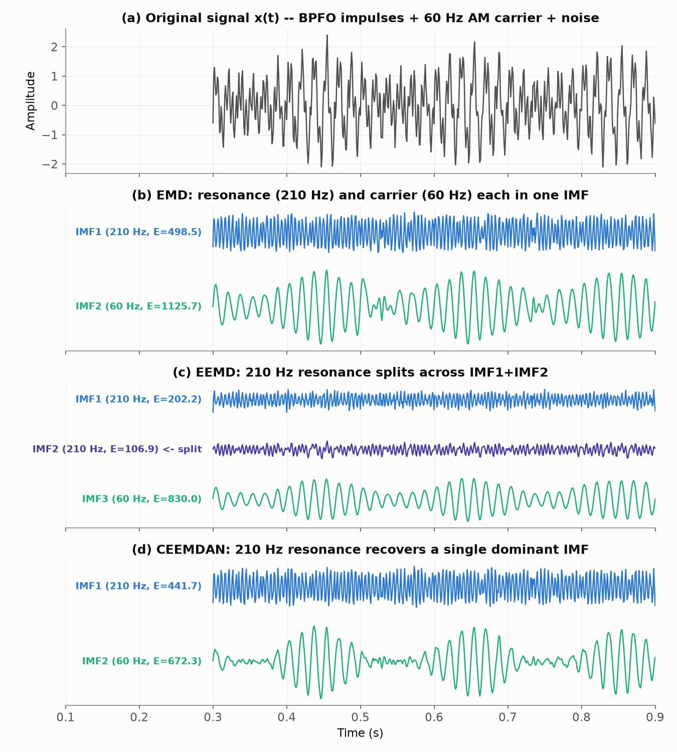
The comparison’s focus is how many IMFs the 210 Hz resonance band is spread across. (b) In EMD, the 210 Hz and 60 Hz components each map to a single IMF. (c) In EEMD, the 210 Hz component splits into IMF1 (E=202.2) and IMF2 (E=106.9) — summing them (202.2+106.9=309.1) only partially recovers the energy of EMD’s single IMF1 (E=498.5), showing that ensemble averaging loses some energy along the way. (d) In CEEMDAN, the 210 Hz component is again concentrated in a single IMF1 (E=441.7), much closer to EMD’s single-IMF structure.
3. The Marginal Hilbert Spectrum
After extracting instantaneous amplitude \(a_k(t)\) and instantaneous frequency \(f_k(t)\) from each IMF via the Hilbert-Huang Transform (see https://yuhi-sa.github.io/en/posts/20260528_mode_decomposition/1/ section 5 and https://yuhi-sa.github.io/en/posts/20260318_hilbert_transform/1/), integrating the energy over time as a function of frequency alone gives the marginal spectrum:
\[ h(f) = \int_0^T \sum_k a_k(t)^2 \, \delta(f - f_k(t)) \, dt \]Unlike the Fourier spectrum, which assumes a fixed frequency content for the entire signal, the marginal spectrum is a time integral of instantaneous frequency, so it represents the energy distribution of non-stationary signals without the smearing that Fourier analysis introduces.
freq_bins = np.linspace(0, fs / 2, 200)
marginal_spectrum = np.zeros_like(freq_bins)

for imf in imfs_ceemdan:
    analytic = hilbert(imf)
    amp = np.abs(analytic)
    phase = np.unwrap(np.angle(analytic))
    inst_freq = np.clip(np.diff(phase) / (2 * np.pi) * fs, 0, fs / 2)
    bin_idx = np.clip(np.digitize(inst_freq, freq_bins) - 1, 0, len(freq_bins) - 1)
    np.add.at(marginal_spectrum, bin_idx, amp[:-1] ** 2)

from scipy.signal import find_peaks
peak_idx, _ = find_peaks(marginal_spectrum, distance=10, prominence=marginal_spectrum.max() * 0.05)
for f, e in sorted(zip(freq_bins[peak_idx], marginal_spectrum[peak_idx]), key=lambda p: -p[1]):
    print(f"peak frequency: {f:.1f} Hz, energy: {e:.1f}")
Result: only two peaks were detected — 60.3 Hz (energy 251.2) and 226.1 Hz (energy 26.4). The 60 Hz AM carrier rings continuously for the full 2 seconds and dominates the marginal spectrum, while the 30 Hz BPFO modulation does not appear as its own peak — because BPFO is not an instantaneous frequency but the period at which the resonance component’s amplitude is modulated, which the marginal spectrum’s definition cannot capture directly. The envelope spectrum method in the next section fills this gap.
4. BPFO Detection via Envelope Spectrum Analysis
Envelope analysis, the standard technique in bearing fault diagnosis, selects the IMF in the resonance band and takes the FFT of its Hilbert envelope (instantaneous amplitude) to recover the period of the impulses exciting the resonance — i.e., the defect frequency.
dom_freqs = [np.fft.rfftfreq(len(imf), 1/fs)[np.argmax(np.abs(np.fft.rfft(imf))[1:]) + 1] for imf in imfs_ceemdan]
resonance_imf_idx = int(np.argmin(np.abs(np.array(dom_freqs) - resonance_freq)))
resonance_imf = imfs_ceemdan[resonance_imf_idx]  # IMF closest to the 200 Hz resonance frequency

envelope = np.abs(hilbert(resonance_imf))
envelope_spec = np.abs(np.fft.rfft(envelope - envelope.mean()))
envelope_freqs = np.fft.rfftfreq(len(envelope), 1 / fs)
bpfo_est = envelope_freqs[np.argmax(envelope_spec)]
print(f"BPFO estimate from envelope spectrum: {bpfo_est:.2f} Hz")
Result: the method automatically selected IMF1 (dominant frequency 210.0 Hz, closest to the 200 Hz resonance), and its envelope spectrum peaked at 30.00 Hz — an exact match to the true 30 Hz. Because CEEMDAN cleanly separates the resonance band from the other components, the downstream envelope analysis works with high precision. With plain EMD, mode mixing can leak AM energy into the resonance band; with EEMD, the resonance band can be split across multiple IMFs, losing information when only a single IMF is selected. This is where CEEMDAN’s practical advantage over both methods shows up directly.
Placing the marginal spectrum and the envelope spectrum side by side makes the difference in their roles visually clear.
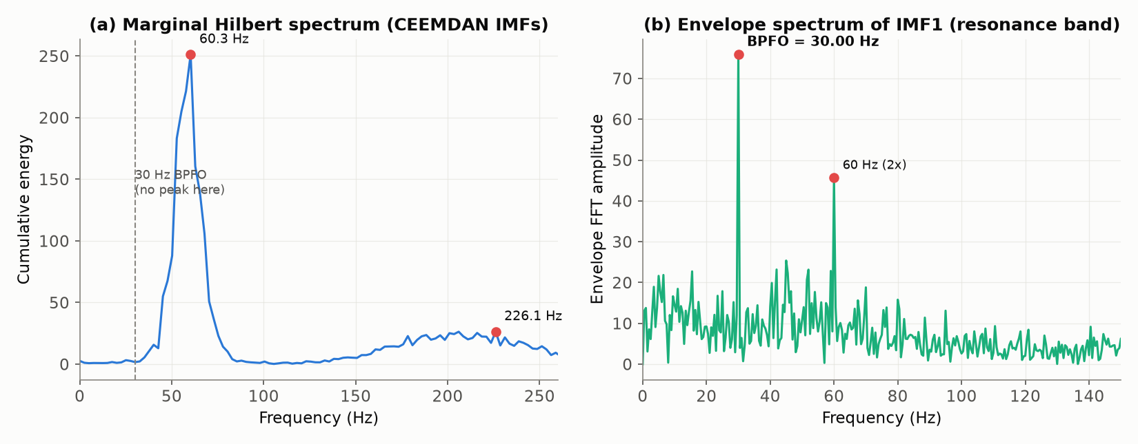
The left panel (marginal spectrum) peaks at 60.3 Hz (the AM carrier) and 226.1 Hz (the residual resonance-band content), but shows nothing at 30 Hz — as discussed in Section 3, the marginal spectrum is a time integral of instantaneous frequency, not a tool for detecting the period of amplitude modulation directly. The right panel (IMF1’s envelope spectrum) shows the opposite: a sharp peak exactly at 30.00 Hz, with its second harmonic visible near 60 Hz. Starting from the same CEEMDAN decomposition, which spectrum you compute determines entirely what information becomes visible — these two panels make that point directly.
4.1 Recent Research in Practice
Combining CEEMDAN with envelope analysis (or its more advanced variants) for bearing diagnosis remains an active research area. For instance, Zhang et al. (2024) propose a wind-turbine bearing fault diagnosis method that decomposes vibration signals with CEEMDAN, then automatically selects the informative IMFs using a composite “KC indicator” combining kurtosis and correlation, followed by multi-scale demodulation via the continuous wavelet transform (CWT) to extract the defect frequency. This replaces the simple selection rule used in this section (picking the single IMF closest to the resonance frequency) with a more robust indicator, and the paper reports improved performance on early-stage faults where impulse amplitudes are small and easily buried in noise (see References for details).
5. When to Use Which Method
| Situation | Recommended | Reason |
|---|---|---|
| Exploratory analysis, computational cost is the priority | EMD | No ensemble needed, fast; mode mixing is tolerable |
| Want to suppress mode mixing but exact reconstruction isn’t needed | EEMD | Simple to implement, widely supported |
| Need precise, quantitative amplitude/energy evaluation downstream | CEEMDAN | Near-zero reconstruction error, better energy conservation |
| Feeding into envelope analysis or similar downstream processing | CEEMDAN | Less mode splitting, resonance band more likely in a single IMF |
All three methods are sensitive to the trials and noise_width/epsilon parameters, so it’s worth running a sensitivity sweep for the SNR of your actual signal before committing to defaults.
6. Learning Checklist
- Explain why EEMD cannot guarantee exact reconstruction, from the non-commutativity of nonlinear operations and averaging
- Write out CEEMDAN’s stage-wise noise-removal procedure as equations
- Distinguish mode mixing from mode splitting
- Explain the difference between the marginal Hilbert spectrum and the Fourier spectrum
- Identify what the marginal spectrum can and cannot detect (e.g., the period of amplitude modulation)
- Implement the envelope spectrum method to estimate bearing fault frequencies (BPFO/BPFI/BSF/FTF)
- Explain the role of the
trials/epsilonparameters inPyEMD.CEEMDAN - Explain CEEMDAN’s stopping criterion (extrema count in the residual) and its practical limitations — endpoint effects and spurious modes at low SNR
Related Articles
- https://yuhi-sa.github.io/en/posts/20260528_mode_decomposition/1/ — EMD, VMD, SSA basics and the mode mixing problem
- https://yuhi-sa.github.io/en/posts/20260318_hilbert_transform/1/ — Hilbert transform and the analytic signal
- https://yuhi-sa.github.io/en/posts/20260714_tkeo/1/ — A lightweight alternative that recovers the same BPFO frequency using only a bandpass filter + TKEO, without any EMD-family decomposition
- https://yuhi-sa.github.io/en/posts/20260524_time_frequency_guide/1/ — Time-frequency analysis method selection hub
- https://yuhi-sa.github.io/en/posts/20260228_timeseries_anomaly/1/ — Anomaly detection in time-series data
- https://yuhi-sa.github.io/en/posts/20260525_ml_timeseries_guide/1/ — Machine learning for time-series forecasting, classification, and anomaly detection
- https://yuhi-sa.github.io/en/posts/20260429_autocorrelation/1/ — Autocorrelation and cross-correlation theory and implementation
References
- Torres, M. E., Colominas, M. A., Schlotthauer, G., & Flandrin, P. (2011). “A complete ensemble empirical mode decomposition with adaptive noise.” 2011 IEEE International Conference on Acoustics, Speech and Signal Processing (ICASSP), 4144-4147. doi:10.1109/ICASSP.2011.5947265
- Huang, N. E., et al. (1998). “The empirical mode decomposition and the Hilbert spectrum for nonlinear and non-stationary time series analysis.” Proceedings of the Royal Society of London A, 454, 903-995.
- Zhang, D., Wang, Y., Jiang, Y., Zhao, T., Xu, H., Qian, P., & Li, C. (2024). “A Novel Wind Turbine Rolling Element Bearing Fault Diagnosis Method Based on CEEMDAN and Improved TFR Demodulation Analysis.” Energies, 17(4), 819. doi:10.3390/en17040819
- PyEMD (EMD-signal) documentation