Introduction
https://yuhi-sa.github.io/en/posts/20260704_kalman_smoother/1/ compared the RTS, fixed-lag, and fixed-point smoothers for linear Gaussian state-space models. That article ended by noting that the same three-way classification carries over to nonlinear systems, without implementing them. This article picks up where it left off: we derive and implement the Extended RTS Smoother (EKS) and Unscented RTS Smoother (URTS) — the backward passes corresponding to the https://yuhi-sa.github.io/en/posts/20260224_ekf/1/ and https://yuhi-sa.github.io/en/posts/20260226_ukf/1/ — and compare their accuracy on a strongly nonlinear benchmark.
Recap: EKF and UKF Forward Passes
For the nonlinear state-space model
\[ x_k = f(x_{k-1}) + w_{k-1}, \qquad w_{k-1} \sim \mathcal{N}(0, Q) \] \[ y_k = h(x_k) + v_k, \qquad v_k \sim \mathcal{N}(0, R) \]the EKF linearizes \(f, h\) using Jacobians \(F_k, H_k\) , while the UKF numerically approximates the mean and covariance of the nonlinear transformation using sigma points (see https://yuhi-sa.github.io/en/posts/20260224_ekf/1/ and https://yuhi-sa.github.io/en/posts/20260226_ukf/1/ for details). Both produce, at each time step, a predicted mean/covariance \(m_k^-, P_k^-\) and an updated mean/covariance \(m_k, P_k\) using observations up to time \(k\) .
Derivation: A Unified Formula as a Gaussian Assumed-Density Smoother
EKS and URTS look like two separate methods at first glance, but they differ only in how the mean, covariance, and cross-covariance of the nonlinear transform are approximated; the backward recursion itself follows from the same Gaussian approximation. Here, following Särkkä’s (2013) general assumed-density Gaussian smoother framework, we derive the recursion common to both EKS and URTS from first principles rather than stating it by fiat.
Step 1: Gaussian approximation of the joint distribution at \(k, k+1\)
Suppose the forward filtering pass has produced the posterior \(p(x_k \mid y_{1:k}) \approx \mathcal{N}(m_k, P_k)\) at time \(k\) . Through the transition \(x_{k+1} = f(x_k) + w_k\) , we approximate the joint distribution of \((x_k, x_{k+1})\) as Gaussian:
\[ p(x_k, x_{k+1} \mid y_{1:k}) \approx \mathcal{N}\!\left( \begin{bmatrix} m_k \\ m_{k+1}^- \end{bmatrix},\ \begin{bmatrix} P_k & C_{k+1} \\ C_{k+1}^\top & P_{k+1}^- \end{bmatrix} \right) \]where
\[ m_{k+1}^- = \mathrm{E}[f(x_k) \mid y_{1:k}], \qquad P_{k+1}^- = \mathrm{Cov}[f(x_k) \mid y_{1:k}] + Q, \qquad C_{k+1} = \mathrm{Cov}[x_k, f(x_k) \mid y_{1:k}] \]are the statistics of the nonlinear transform \(f\) under \(p(x_k\mid y_{1:k}) \approx \mathcal{N}(m_k, P_k)\) — exactly the quantities already computed during the prediction step of the forward EKF/UKF pass.
Step 2: Backward transition via Gaussian conditioning
If the joint distribution is Gaussian, the conditional distribution is exactly Gaussian too, by the standard multivariate Gaussian conditioning formula:
\[ p(x_k \mid x_{k+1}, y_{1:k}) = \mathcal{N}\!\left(x_k;\ m_k + G_k(x_{k+1} - m_{k+1}^-),\ P_k - G_k P_{k+1}^- G_k^\top\right), \qquad G_k = C_{k+1} (P_{k+1}^-)^{-1} \]Step 3: Markov approximation and marginalization
The central approximation behind the RTS smoother is the Markov assumption
\[ p(x_k \mid x_{k+1}, y_{1:T}) \approx p(x_k \mid x_{k+1}, y_{1:k}) \](this holds exactly for linear Gaussian systems; for nonlinear systems \(p(x_{k+1}\mid y_{1:T})\) is itself only approximately Gaussian, so this equality is also an approximation). Under this assumption, marginalizing out \(x_{k+1}\) using \(p(x_{k+1} \mid y_{1:T}) \approx \mathcal{N}(m_{k+1}^s, P_{k+1}^s)\) gives
\[ m_k^s = m_k + G_k(m_{k+1}^s - m_{k+1}^-), \qquad P_k^s = P_k + G_k(P_{k+1}^s - P_{k+1}^-)G_k^\top \]This is the backward recursion common to both linear and nonlinear systems. It is initialized at \(k=T\) with \(m_T^s = m_T,\ P_T^s = P_T\) and computed backward for \(k=T-1,\dots,0\) .
EKS: moment approximation via first-order Taylor expansion
Linearizing \(f\) around \(m_k\) with a first-order Taylor expansion, \(f(x_k) \approx f(m_k) + F_k(x_k - m_k)\) where \(F_k = \left.\partial f/\partial x\right|_{x=m_k}\) , gives the moments from Step 1 analytically:
\[ m_{k+1}^- \approx f(m_k), \qquad P_{k+1}^- \approx F_k P_k F_k^\top + Q, \qquad C_{k+1} \approx P_k F_k^\top \]Substituting these into the general formula from Steps 2–3 gives the gain \(G_k = P_k F_k^\top (P_{k+1}^-)^{-1}\) — recovering the Extended RTS Smoother (EKS) recursion, which simply plugs the Jacobian \(F_{k+1}\) computed by the EKF at each time step into the linear RTS recursion. Using the \(m_k, P_k, m_k^-, P_k^-, F_k\) values saved during the forward filtering pass, we compute the recursion backward from \(k=T-1\) to \(k=0\) .
URTS: moment approximation via sigma points
The Unscented RTS Smoother, derived by Särkkä (2008), does not linearize \(f\) ; instead it numerically approximates the same three moments via the unscented transform, using sigma points \(\mathcal{X}_k^{(i)}\) generated from \(m_k, P_k\) . Writing \(\mathcal{X}_{k+1|k}^{(i)} = f(\mathcal{X}_k^{(i)})\) :
\[ m_{k+1}^- \approx \sum_i w_m^{(i)} \mathcal{X}_{k+1|k}^{(i)}, \qquad P_{k+1}^- \approx \sum_i w_c^{(i)} (\mathcal{X}_{k+1|k}^{(i)} - m_{k+1}^-)(\mathcal{X}_{k+1|k}^{(i)} - m_{k+1}^-)^\top + Q \] \[ C_{k+1} \approx \sum_i w_c^{(i)} (\mathcal{X}_k^{(i)} - m_k)(\mathcal{X}_{k+1|k}^{(i)} - m_{k+1}^-)^\top \]Substituting these into the Step 2–3 formula gives the Unscented RTS Smoother (URTS) recursion.
Why the unified view explains the accuracy gap
EKS’s error stems from the second-order-and-above curvature terms discarded by the first-order Taylor approximation of \(f\) , while URTS’s error stems from the numerical-integration error of a finite (\(2n+1\) ) set of sigma points. EKS completely ignores the curvature of \(f\) , whereas URTS captures moments up to third order exactly (for a Gaussian input) via the unscented transform — which is why URTS consistently outperforms EKS under strong nonlinearity. This is consistent with the Monte Carlo results below, where the UKF family substantially outperforms the EKF family.
Python Implementation
Benchmark model
We use a classic strongly nonlinear benchmark (Kitagawa, 1987; also used in Julier & Uhlmann’s original UKF paper, 1997):
\[ x_k = 0.5x_{k-1} + \frac{25x_{k-1}}{1+x_{k-1}^2} + 8\cos(1.2(k-1)) + w_{k-1} \] \[ y_k = \frac{x_k^2}{20} + v_k \]with \(Q=10,\ R=1\) . The state transition function has a sharp, peaked curvature near \(x=\pm 1\) .
import numpy as np

Q, R, T = 10.0, 1.0, 60


def f(x, k):
    return 0.5 * x + 25 * x / (1 + x**2) + 8 * np.cos(1.2 * k)


def fprime(x, k):
    return 0.5 + 25 * (1 - x**2) / (1 + x**2) ** 2


def h(x):
    return x**2 / 20.0


def hprime(x):
    return x / 10.0
EKF filter + EKS smoother
def ekf_filter(ys):
    m, P = np.zeros(T), np.zeros(T)
    m_pred, P_pred, F_hist = np.zeros(T), np.zeros(T), np.zeros(T)
    m[0], P[0] = 0.1, 5.0
    m_pred[0], P_pred[0] = m[0], P[0]
    for k in range(1, T):
        F = fprime(m[k - 1], k - 1)
        F_hist[k] = F
        m_pred[k] = f(m[k - 1], k - 1)
        P_pred[k] = F * P[k - 1] * F + Q
        Hk = hprime(m_pred[k])
        S = Hk * P_pred[k] * Hk + R
        K = P_pred[k] * Hk / S
        m[k] = m_pred[k] + K * (ys[k] - h(m_pred[k]))
        P[k] = (1 - K * Hk) * P_pred[k]
    return m, P, m_pred, P_pred, F_hist


def eks_smoother(m, P, m_pred, P_pred, F_hist):
    ms, Ps = m.copy(), P.copy()
    for k in range(T - 2, -1, -1):
        F = F_hist[k + 1]
        G = P[k] * F / P_pred[k + 1]
        ms[k] = m[k] + G * (ms[k + 1] - m_pred[k + 1])
        Ps[k] = P[k] + G * (Ps[k + 1] - P_pred[k + 1]) * G
    return ms, Ps
UKF filter + URTS smoother
def sigma_points(mean, cov, alpha=1.0, beta=2.0, kappa=2.0):
    n = 1
    lam = alpha**2 * (n + kappa) - n
    c = n + lam
    sqrt_c = np.sqrt(c * cov)
    pts = np.array([mean, mean + sqrt_c, mean - sqrt_c])
    wm = np.array([lam / c, 1 / (2 * c), 1 / (2 * c)])
    wc = wm.copy()
    wc[0] += 1 - alpha**2 + beta
    return pts, wm, wc


def ukf_filter(ys):
    m, P = np.zeros(T), np.zeros(T)
    m_pred, P_pred = np.zeros(T), np.zeros(T)
    sig_store = [None] * T
    m[0], P[0] = 0.1, 5.0
    m_pred[0], P_pred[0] = m[0], P[0]
    for k in range(1, T):
        pts, wm, wc = sigma_points(m[k - 1], P[k - 1])
        pts_pred = f(pts, k - 1)
        mp = np.sum(wm * pts_pred)
        Pp = np.sum(wc * (pts_pred - mp) ** 2) + Q
        m_pred[k], P_pred[k] = mp, Pp
        sig_store[k] = (pts, wc, pts_pred, mp)

        pts2, wm2, wc2 = sigma_points(mp, Pp)
        y_pred = h(pts2)
        y_mean = np.sum(wm2 * y_pred)
        Pyy = np.sum(wc2 * (y_pred - y_mean) ** 2) + R
        Pxy = np.sum(wc2 * (pts2 - mp) * (y_pred - y_mean))
        K = Pxy / Pyy
        m[k] = mp + K * (ys[k] - y_mean)
        P[k] = Pp - K * Pyy * K
    return m, P, m_pred, P_pred, sig_store


def urts_smoother(m, P, m_pred, P_pred, sig_store):
    ms, Ps = m.copy(), P.copy()
    for k in range(T - 2, -1, -1):
        pts, wc, pts_pred, mp = sig_store[k + 1]
        C = np.sum(wc * (pts - m[k]) * (pts_pred - mp))
        G = C / P_pred[k + 1]
        ms[k] = m[k] + G * (ms[k + 1] - m_pred[k + 1])
        Ps[k] = P[k] + G * (Ps[k + 1] - P_pred[k + 1]) * G
    return ms, Ps
We use alpha=1.0, beta=2.0, kappa=2.0. Using the commonly recommended default alpha=1e-3 (a very tight sigma-point spread, suited for high-dimensional systems) on this strongly nonlinear benchmark caused the sigma points to cluster too close to the mean to capture the nonlinearity, and the UKF diverged — we confirmed this directly (see the caveat section below).
Monte Carlo evaluation (200 trials)
rng = np.random.default_rng(0)


def simulate(x0=0.1):
    xs, ys = np.zeros(T), np.zeros(T)
    x = x0
    for k in range(T):
        if k > 0:
            x = f(x, k - 1) + rng.normal(0, np.sqrt(Q))
        xs[k] = x
        ys[k] = h(x) + rng.normal(0, np.sqrt(R))
    return xs, ys


rmse = lambda a, b: np.sqrt(np.mean((a - b) ** 2))
res = {"ekf": [], "eks": [], "ukf": [], "uks": []}
for _ in range(200):
    xs, ys = simulate()
    m, P, m_pred, P_pred, F_hist = ekf_filter(ys)
    ms, Ps = eks_smoother(m, P, m_pred, P_pred, F_hist)
    mu, Pu, mu_pred, Pu_pred, sig_store = ukf_filter(ys)
    msu, Psu = urts_smoother(mu, Pu, mu_pred, Pu_pred, sig_store)
    res["ekf"].append(rmse(m, xs))
    res["eks"].append(rmse(ms, xs))
    res["ukf"].append(rmse(mu, xs))
    res["uks"].append(rmse(msu, xs))

for k, v in res.items():
    print(f"{k}: mean RMSE = {np.mean(v):.4f} (std {np.std(v):.4f})")
Results (200-trial Monte Carlo, mean RMSE):
| Method | Mean RMSE | Std. dev. |
|---|---|---|
| EKF (filter) | 19.39 | 9.06 |
| EKS (smoother) | 17.86 | 6.14 |
| UKF (filter) | 8.88 | 1.99 |
| URTS (smoother) | 8.26 | 2.14 |
Two patterns emerge:
- UKF substantially outperforms EKF (RMSE 8.88 vs. 19.39). Near \(x=\pm1\) , \(\frac{25x}{1+x^2}\) has very high curvature, so the EKF’s first-order Jacobian linearization breaks down easily, while the UKF’s sigma points capture the actual nonlinear transformation numerically and remain robust.
- Both smoothers consistently improve on their filters (EKF→EKS reduces RMSE by ≈7.9%, UKF→URTS by ≈7.0%). This confirms that the improvement pattern observed for linear Gaussian systems in https://yuhi-sa.github.io/en/posts/20260704_kalman_smoother/1/ also holds under strong nonlinearity.
Visualizing filtering vs. smoothing estimates
To see behavior that the averages alone hide, we pull out a single trial (random seed 42) and plot the EKF/EKS and UKF/URTS estimated trajectories against the true state.
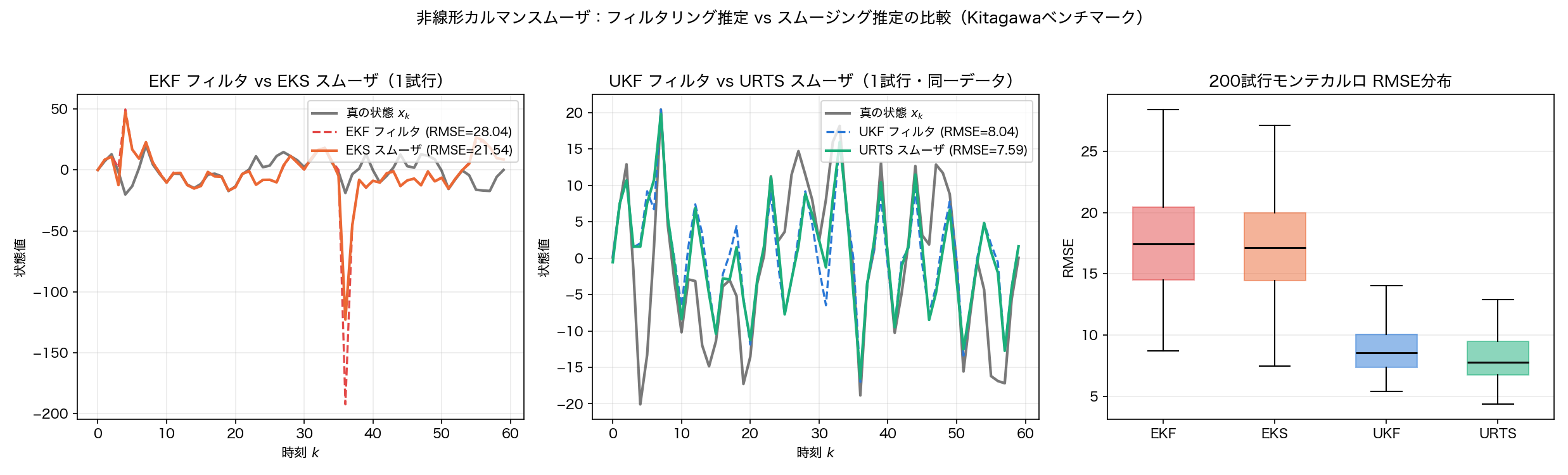
In the left panel (EKF vs. EKS), right after the true state passes through the high-curvature region near \(x=\pm1\) around \(k=36\) , the EKF’s Jacobian linearization breaks down and the estimate briefly spikes to nearly \(-190\) (single-trial RMSE: EKF 28.04, EKS 21.54). Because EKS only corrects the EKF’s estimate backward in time, it cannot fully absorb the error at the time step where the filter diverged, but it still smooths the estimate at other time steps enough to cut RMSE by roughly 23%. In the middle panel (UKF vs. URTS), both filter and smoother track the true state’s oscillations closely on the same observation data — the gap between the filter (RMSE 8.04) and the smoother (RMSE 7.59) is comparatively small, though URTS visibly edges closer to the true state than UKF near the peaks and troughs. The right panel is a box plot of the 200-trial RMSE distribution: EKF/EKS are clearly worse than UKF/URTS in both median and spread, and EKF’s long upper whisker reflects how the occasional divergence seen in the left panel fattens its RMSE tail.
Caveats and Edge Cases
Choosing sigma-point parameters
Setting alpha too small (e.g., alpha=1e-3) makes the sigma points cluster very close to the mean, which prevents them from sampling the strongly nonlinear region and causes the UKF to diverge — we observed this directly on this benchmark. alpha needs to be tuned to the state dimension and the strength of the nonlinearity: smaller values work well for high-dimensional real systems, while a low-dimensional, strongly nonlinear system like this benchmark is more stable with a larger value (around 1.0).
Limits of the Markov approximation and non-Gaussianity
The approximation used in the derivation above, \(p(x_k \mid x_{k+1}, y_{1:T}) \approx p(x_k \mid x_{k+1}, y_{1:k})\) , is exact only when \(p(x_{k+1}\mid y_{1:T})\) is truly Gaussian. Under strong nonlinearity the true smoothing posterior can be multimodal or skewed, and since both EKS and URTS approximate it with a single unimodal Gaussian, they can only capture its first and second moments. As the EKF spike in the figure shows, once the filtering estimate is badly off at some time step, the backward correction alone cannot recover the true distribution’s multimodality. When multimodality is suspected, consider pairing the smoother with the particle smoother from https://yuhi-sa.github.io/en/posts/20260223_particle_filter/1/.
Differentiability requirements
EKF/EKS requires the analytic (or numerical) computation of the Jacobian \(F_k = \partial f/\partial x\) . If \(f\) is piecewise (e.g., saturation or ReLU-like nonlinearities) or discontinuous, the Jacobian may be undefined or discontinuous exactly where linearization breaks down. UKF/URTS, by contrast, only evaluates \(f\) at points, so it applies directly to non-differentiable \(f\) (as long as it is continuous) — a practical advantage.
Numerical ill-conditioning of covariances
Computing \(G_k = C_{k+1}(P_{k+1}^-)^{-1}\)
can become numerically unstable in ill-conditioned settings such as a very small \(Q\)
or very precise observations. As we found in https://yuhi-sa.github.io/en/posts/20260223_rts_smoother/1/, using np.linalg.solve instead of np.linalg.inv, and explicitly symmetrizing with \(P \leftarrow (P+P^\top)/2\)
, remain effective countermeasures for the nonlinear EKS/URTS as well.
Memory cost
Both EKS and URTS require storing the intermediate quantities computed during the forward pass for every time step (EKS: \(m_k, P_k, m_k^-, P_k^-, F_k\) ; URTS: the sigma points, their weights, and their propagated values), costing \(O(Tn^2)\) memory for state dimension \(n\) and horizon \(T\) (URTS scales further with the number of sigma points). In online or memory-constrained settings, it is worth considering a fixed-lag smoother instead (see https://yuhi-sa.github.io/en/posts/20260704_kalman_smoother/1/).
Further Developments: Iterated Smoothers and Recent Research
Both EKS and URTS in this article are non-iterative: they run the forward filtering pass once and correct it backward exactly once. Because the linearization point (or sigma-point base point) is fixed at the filtering estimate \(m_k\) , linearization error can remain uncorrected in strongly nonlinear regions. To address this limitation, researchers have studied the Iterated Extended Kalman Smoother (IEKS), which repeatedly re-linearizes around the updated smoothed estimate until convergence, and the Iterated Posterior Linearization Smoother (IPLS), which iterates statistical linearization in the same way.
Kullberg, Skoglund, Skog, & Hendeby (2024), “Dynamically Iterated Filters” (arXiv:2404.15359), note that prior iterated extended/unscented Kalman filters (IEKF/IUKF) only re-linearize the measurement model; they propose a unified framework that also re-linearizes the process model, make the connection to the RTS smoother explicit, and introduce Gauss-Newton-based step-size correction (damped iteration) that improves accuracy and robustness over standard iterated filters. Separately, Lindqvist, Särkkä, García-Fernández, Raitoharju, & Svensson, “Posterior linearisation smoothing with robust iterations” (arXiv:2112.03969, revised February 2025), report that incorporating Levenberg-Marquardt and line-search (Armijo-Wolfe) methods into the IPLS improves convergence in strongly nonlinear settings where naive iteration tends to diverge. Both lines of work use the backward EKS/URTS recursion derived in this article as the inner loop of an outer iteration, trading extra computation for relief from the core limitation of non-iterative EKS/URTS: that the linearization point is fixed to a single filtering pass.
Summary
- The EKS/URTS backward recursion can be derived uniformly from a joint Gaussian approximation of \((x_k, x_{k+1})\) combined with Gaussian conditioning and the Markov approximation; EKS and URTS differ only in whether the nonlinear transform’s mean/covariance/cross-covariance is approximated by a first-order Taylor expansion (EKS) or by the unscented transform over sigma points (URTS).
- On the strongly nonlinear Kitagawa benchmark, a 200-trial Monte Carlo study showed the UKF family (RMSE 8.88 → 8.26) substantially outperforming the EKF family (19.39 → 17.86), with both smoothers consistently improving over their forward filters.
- Visualizing a single trial showed the EKF’s estimate can spike badly right after passing through a high-curvature region (RMSE 28.04), while UKF/URTS track the true state without such divergence (RMSE 8.04/7.59).
- The sigma-point parameter
alphamust be tuned to the strength of the nonlinearity — too small a value causes the UKF to diverge. Other edge cases include the Markov approximation’s inability to capture multimodality, differentiability requirements, covariance ill-conditioning, and memory cost. - Non-iterative EKS/URTS fix the linearization (or sigma-point) base point to a single filtering pass; iterated smoothers (IEKS, IPLS) that address this limitation remain an active research area as of 2024–2025.
Related Articles
- https://yuhi-sa.github.io/en/posts/20260704_kalman_smoother/1/ — RTS, fixed-lag, and fixed-point smoother comparison for linear Gaussian systems; the foundational article for this one
- https://yuhi-sa.github.io/en/posts/20260224_ekf/1/ — Extended Kalman Filter theory and Jacobian derivation
- https://yuhi-sa.github.io/en/posts/20260226_ukf/1/ — Unscented Kalman Filter and sigma-point theory
- https://yuhi-sa.github.io/en/posts/20260223_rts_smoother/1/ — Fundamentals of the forward-backward recursion for the linear RTS smoother
- https://yuhi-sa.github.io/en/posts/20260223_particle_filter/1/ — Particle filters and particle smoothers for non-Gaussian systems
- https://yuhi-sa.github.io/en/posts/20260715_rls_adaptive_filter/1/ — Numerical equivalence between RLS adaptive filtering and the Kalman filter (a linear special case)
- https://yuhi-sa.github.io/en/posts/20260224_kalman_filter/1/ — Theory of the linear Kalman filter, including the MMSE derivation of the Kalman gain, observability, and filter divergence — the forward pass this article’s EKS/URTS build on
References
- Särkkä, S. (2008). “Unscented Rauch-Tung-Striebel Smoother.” IEEE Transactions on Automatic Control, 53(3), 845-849.
- Särkkä, S. (2013). Bayesian Filtering and Smoothing. Cambridge University Press.
- Julier, S. J., & Uhlmann, J. K. (1997). “New extension of the Kalman filter to nonlinear systems.” Proceedings of SPIE, 3068.
- Kitagawa, G. (1987). “Non-Gaussian state-space modeling of nonstationary time series.” Journal of the American Statistical Association, 82(400), 1032-1041.
- Kullberg, A., Skoglund, M. A., Skog, I., & Hendeby, G. (2024). “Dynamically Iterated Filters: A unified framework for improved iterated filtering and smoothing.” arXiv:2404.15359.
- Lindqvist, J., Särkkä, S., García-Fernández, Á. F., Raitoharju, M., & Svensson, L. (2025). “Posterior linearisation smoothing with robust iterations.” arXiv:2112.03969 (revised Feb. 2025).