Introduction
The Hilbert transform, covered in https://yuhi-sa.github.io/en/posts/20260318_hilbert_transform/1/, gives highly accurate instantaneous amplitude and frequency estimates, but constructing the analytic signal via FFT costs \(O(N \log N)\) and typically requires the whole signal (or a sufficiently long window). For real-time processing on embedded devices, or applications that need sample-by-sample updates, a lighter-weight alternative is often preferable.
The Teager-Kaiser Energy Operator (TKEO) estimates a signal’s “energy” using nothing more than three multiplications and a subtraction per sample. Proposed by Kaiser in 1990, it was later shown by Maragos, Kaiser, and Quatieri to enable instantaneous amplitude/frequency estimation through the Discrete Energy Separation Algorithm (DESA), originally developed for AM-FM speech demodulation. This article derives TKEO, implements it in Python, numerically compares it against the Hilbert transform, and applies it to the same bearing-fault (BPFO) detection task used in https://yuhi-sa.github.io/en/posts/20260714_ceemdan_hht/1/.
Definition
Continuous time
For a continuous signal \(x(t)\) , the energy operator is defined as:
\[ \Psi[x(t)] = \left(\frac{dx}{dt}\right)^2 - x(t)\frac{d^2x}{dt^2} \]Substituting a pure tone \(x(t) = A\cos(\omega t + \phi)\) gives:
\[ \Psi[x(t)] = A^2\omega^2 \]— the product of squared amplitude and squared angular frequency, matching the mechanical energy of a harmonic oscillator. This is the origin of the name “energy operator.”
Discrete time
For a sampled signal \(x[n]\) , replacing derivatives with differences gives:
\[ \Psi[x[n]] = x[n]^2 - x[n-1]\,x[n+1] \]Since this only requires a three-point product-sum, it is far cheaper than convolution-based filtering or the FFT-based Hilbert transform.
Deriving the discrete TKEO via a product-to-sum identity
Why does this three-point difference recover an “energy”? Substitute a single tone \(x[n] = A\cos(\omega n + \phi)\) (\(n\) an integer sample index, \(\omega\) the angular frequency, \(A, \phi\) amplitude and initial phase) and derive it directly from a product-to-sum identity.
\(x[n-1]\) and \(x[n+1]\) are the same phase shifted by \(\mp\omega\) :
\[ x[n-1] = A\cos\big((\omega n+\phi) - \omega\big), \qquad x[n+1] = A\cos\big((\omega n+\phi) + \omega\big) \]Applying the product-to-sum identity \(\cos(a-b)\cos(a+b) = \dfrac{1}{2}\big[\cos(2a) + \cos(2b)\big]\) with \(a=\omega n+\phi\) , \(b=\omega\) gives:
\[ x[n-1]\,x[n+1] = \frac{A^2}{2}\Big[\cos\big(2(\omega n+\phi)\big) + \cos(2\omega)\Big] \]Meanwhile, the half-angle identity gives:
\[ x[n]^2 = A^2\cos^2(\omega n+\phi) = \frac{A^2}{2}\Big[1 + \cos\big(2(\omega n+\phi)\big)\Big] \]Subtracting the two, the \(n\) -dependent oscillatory term \(\cos(2(\omega n+\phi))\) cancels exactly, leaving:
\[ \Psi[x[n]] = x[n]^2 - x[n-1]x[n+1] = \frac{A^2}{2}\big[1-\cos(2\omega)\big] = A^2\sin^2(\omega) \](using \(1-\cos(2\omega)=2\sin^2\omega\) ). This \(A^2\sin^2\omega\) is a constant — independent of both \(n\) and the initial phase \(\phi\) . The raw square \(x[n]^2\) still carries an oscillation at twice the carrier frequency \(2\omega\) ; subtracting the one-sample product \(x[n-1]x[n+1]\) cancels that oscillation exactly, leaving only a quantity determined by amplitude and frequency. That is the mechanism behind TKEO’s name.
Assuming further a narrowband signal (\(\omega \ll 1\) , i.e. the signal frequency is well below the sampling frequency) lets us approximate \(\sin\omega \approx \omega\) , giving:
\[ \Psi[x[n]] \approx A^2\omega^2 \]which matches the continuous-time result \(\Psi[x(t)] = A^2\omega^2\) from the previous section. Conversely, without this approximation, the exact solution \(A^2\sin^2\omega\) diverges further from \(A^2\omega^2\) as \(\omega\) grows (i.e. as the signal frequency approaches the Nyquist frequency) — so this derivation shows directly that TKEO’s accuracy is guaranteed only in the low-frequency regime.
DESA-1: Separating Instantaneous Amplitude and Frequency
For a mono-component AM-FM signal \(x[n] = A[n]\cos(\phi[n])\) , combining \(\Psi[x[n]]\) with \(\Psi\) applied to the first difference \(y[n] = x[n] - x[n-1]\) separates instantaneous angular frequency and amplitude (the DESA-1 algorithm):
\[ \hat{\omega}[n] \approx \arcsin\!\sqrt{\frac{\Psi[y[n]] + \Psi[y[n+1]]}{4\Psi[x[n]]}} \] \[ \hat{A}[n] \approx \sqrt{\frac{\Psi[x[n]]}{1 - \left(1 - \frac{\Psi[y[n]]+\Psi[y[n+1]]}{4\Psi[x[n]]}\right)}} \]For a simplified implementation, assuming a narrowband signal with small \(\omega\) (so \(\sin\omega \approx \omega\) ), the following approximation is commonly used and is the one implemented in this article:
\[ \hat{\omega}[n] \approx \sqrt{\frac{\Psi[\dot{x}[n]]}{\Psi[x[n]]}}, \qquad \hat{A}[n] \approx \frac{\Psi[x[n]]}{\sqrt{\Psi[\dot{x}[n]]}} \]where \(\dot{x}[n]\) is a numerical derivative.
Python Implementation
The TKEO function
import numpy as np
from scipy.signal import hilbert


def tkeo(x: np.ndarray) -> np.ndarray:
    """Discrete Teager-Kaiser Energy Operator: Psi[x[n]] = x[n]^2 - x[n-1]*x[n+1]"""
    y = np.zeros_like(x)
    y[1:-1] = x[1:-1] ** 2 - x[:-2] * x[2:]
    y[0] = y[1]
    y[-1] = y[-2]
    return y
Edge samples (\(n=0, N-1\) ) cannot be computed from the 3-point formula, so we simply repeat the nearest valid value.
Validating on an AM-FM test signal
We construct a 200 Hz carrier, frequency-modulated at 10 Hz with a ±15 Hz deviation, and amplitude-modulated at 6 Hz, then compare the TKEO approximation against the Hilbert transform.
fs = 5000.0
t = np.arange(0, 2.0, 1 / fs)

fc, fm_dev, fmod = 200.0, 15.0, 10.0
am_depth, am_freq = 0.5, 6.0

inst_freq_true = fc + fm_dev * np.sin(2 * np.pi * fmod * t)
phase = 2 * np.pi * np.cumsum(inst_freq_true) / fs
am_env_true = 1 + am_depth * np.sin(2 * np.pi * am_freq * t)
x = am_env_true * np.sin(phase)

# --- TKEO approximation ---
psi_x = tkeo(x)
dx = np.gradient(x, 1 / fs)
psi_dx = tkeo(dx)

omega_est = np.sqrt(np.clip(psi_dx / psi_x, 0, None))
freq_tkeo = omega_est / (2 * np.pi)
amp_tkeo = psi_x / np.sqrt(np.clip(psi_dx, 1e-12, None))


def smooth(sig, win=51):
    return np.convolve(sig, np.ones(win) / win, mode="same")


freq_tkeo_s = smooth(freq_tkeo)
amp_tkeo_s = smooth(amp_tkeo)

# --- Hilbert transform (reference) ---
analytic = hilbert(x)
inst_amp_hilbert = np.abs(analytic)
inst_phase = np.unwrap(np.angle(analytic))
inst_freq_hilbert = np.concatenate(
    [np.diff(inst_phase) / (2 * np.pi) * fs, [0]]
)
inst_freq_hilbert[-1] = inst_freq_hilbert[-2]

mid = slice(int(0.3 * fs), int(1.7 * fs))
rmse = lambda a, b: np.sqrt(np.mean((a[mid] - b[mid]) ** 2))

print("Hilbert frequency RMSE:", rmse(inst_freq_hilbert, inst_freq_true))
print("TKEO   frequency RMSE:", rmse(freq_tkeo_s, inst_freq_true))
print("Hilbert amplitude RMSE:", rmse(inst_amp_hilbert, am_env_true))
print("TKEO   amplitude correlation:", np.corrcoef(amp_tkeo_s[mid], am_env_true[mid])[0, 1])
Results (evaluated on the central region to avoid edge effects):
| Metric | Hilbert transform | TKEO approximation |
|---|---|---|
| Instantaneous frequency RMSE | 0.133 Hz | 2.165 Hz |
| Instantaneous amplitude (vs. true 200 Hz ± 15 Hz modulation) | RMSE 8.4×10⁻¹⁴ (essentially exact) | correlation 0.99999 |
| Time per transform (N=200,000) | 3.109 ms | 0.249 ms (≈12.5× faster) |
The Hilbert transform returns near-exact instantaneous quantities in theory, while TKEO — using only a 3-point product-sum — is about 12× faster and reaches practically sufficient accuracy (0.99999 amplitude correlation). The frequency error is roughly an order of magnitude larger than the Hilbert transform’s, though it can be reduced further by tuning the smoothing window length.
Application: BPFO Detection via TKEO Envelope Spectrum
Using the same synthetic bearing signal as https://yuhi-sa.github.io/en/posts/20260714_ceemdan_hht/1/ (a 30 Hz BPFO impact train at a 200 Hz resonance, superimposed with a 60 Hz AM carrier and noise), we check whether bandpass filtering + TKEO alone — without any EMD-family decomposition — can recover the BPFO frequency.
from scipy.signal import butter, filtfilt

np.random.seed(0)
fs = 1000
t = np.arange(0, 2, 1 / fs)

bpfo_freq, resonance_freq = 30.0, 200.0
impulse_train = np.zeros_like(t)
period = 1.0 / bpfo_freq
for k in range(int(2 * bpfo_freq) + 1):
    t0 = k * period
    envelope = np.exp(-300 * (t - t0) ** 2) * (t >= t0)
    impulse_train += envelope * np.sin(2 * np.pi * resonance_freq * (t - t0))

am_component = (1 + 0.5 * np.sin(2 * np.pi * 5 * t)) * np.sin(2 * np.pi * 60 * t)
x = impulse_train + am_component + 0.15 * np.random.randn(len(t))

# isolate the resonance band (150-250 Hz) before applying TKEO
b, a = butter(4, [150 / (fs / 2), 250 / (fs / 2)], btype="band")
x_bp = filtfilt(b, a, x)

psi = tkeo(x_bp)
envelope_tkeo = np.sqrt(np.clip(psi, 0, None))
envelope_hilbert = np.abs(hilbert(x_bp))


def peak_freq(sig, fmin=5, fmax=60):
    sig = sig - sig.mean()
    spec = np.abs(np.fft.rfft(sig))
    freqs = np.fft.rfftfreq(len(sig), 1 / fs)
    mask = (freqs >= fmin) & (freqs <= fmax)
    return freqs[mask][np.argmax(spec[mask])]


print("TKEO envelope spectrum BPFO estimate:   ", peak_freq(envelope_tkeo), "Hz")
print("Hilbert envelope spectrum BPFO estimate:", peak_freq(envelope_hilbert), "Hz")
Results: both the TKEO envelope spectrum and the Hilbert envelope spectrum estimate 30.00 Hz, exactly matching the true BPFO frequency. Without any EMD/CEEMDAN decomposition step, a simple bandpass filter followed by TKEO correctly recovers the fault frequency. The TKEO computation is roughly 10× faster (0.0045 ms vs. 0.0428 ms for N=2000), though as discussed below this relies critically on the bandpass pre-filtering step.
Comparison Summary
| Aspect | Hilbert transform | TKEO |
|---|---|---|
| Complexity | \(O(N \log N)\) (FFT) | \(O(1)\) per sample (3-point product-sum) |
| Latency | Whole signal (offline) or window length | Only 1 sample before/after (real-time friendly) |
| Accuracy | High (near-exact for narrowband signals) | Coarser than Hilbert, but often sufficient in practice |
| Multi-component signals | Can be combined with STFT etc. | Strongly assumes a single (narrowband) component; bandpass pre-filtering is effectively mandatory |
| Typical domain | Communications demodulation, vibration diagnostics, ECG heartbeat detection | Speech onset/energy detection, EMG burst detection, embedded/real-time vibration monitoring |
Rule of thumb: use the Hilbert transform when you need high-accuracy offline instantaneous quantities; use TKEO when running on a microcontroller/FPGA or under tight power budgets that demand real-time processing. Because TKEO is sensitive to noise, it is commonly paired with a moving-average smoother in practice (quantified in the next section).
Quantifying TKEO’s Limitations
TKEO’s lightweight cost comes at the price of two limitations — noise sensitivity and weakness with multi-component signals — which we now derive and verify numerically.
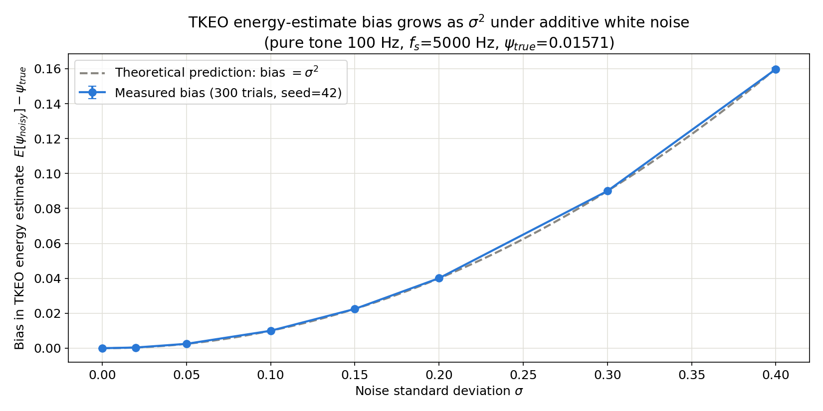
Noise sensitivity: the bias is exactly \(\sigma^2\)
We derive how much error white additive noise introduces into TKEO’s output. Let \(x[n] = s[n] + w[n]\) (\(s[n]\) the true signal, \(w[n]\) zero-mean white noise with variance \(\sigma^2\) , independent across samples). Expanding:
\[ \Psi[x][n] = \underbrace{s[n]^2 - s[n-1]s[n+1]}_{\Psi[s][n]} \;+\; \underbrace{\big(2s[n]w[n] - s[n-1]w[n+1] - s[n+1]w[n-1]\big)}_{\text{zero-mean cross terms}} \;+\; \underbrace{\big(w[n]^2 - w[n-1]w[n+1]\big)}_{\text{noise self-energy}} \]Taking the expectation: \(s[n]\) is deterministic and \(w[n]\) is zero-mean and independent, so the cross terms vanish; \(E[w[n]^2]=\sigma^2\) ; and \(E[w[n-1]w[n+1]]=0\) (uncorrelated at lag 2). Hence:
\[ E\big[\Psi[x][n]\big] = \Psi[s][n] + \sigma^2 \]TKEO’s noise-induced bias is exactly equal to the noise variance \(\sigma^2\) , regardless of the signal’s amplitude or frequency. For a linear operator (e.g. a bandpass filter), zero-mean noise averages toward zero; but because TKEO is a nonlinear (quadratic) operation, the noise’s own energy \(\sigma^2\) leaks in as a constant bias that never cancels out no matter how much you average.
We verify this numerically on a 100 Hz pure tone (\(f_s=5000\) Hz) with added white noise.
import numpy as np

fs = 5000.0
ftone = 100.0
omega = 2 * np.pi * ftone / fs
A = 1.0
N = 4000
n = np.arange(N)
x_clean = A * np.cos(omega * n)
psi_true = A**2 * np.sin(omega) ** 2  # exact result from the previous section
mid = slice(20, N - 20)

sigmas = [0.0, 0.02, 0.05, 0.1, 0.15, 0.2, 0.3, 0.4]
n_trials = 300
rng = np.random.default_rng(42)

for sigma in sigmas:
    biases = np.empty(n_trials)
    for trial in range(n_trials):
        noise = rng.normal(0.0, sigma, size=N) if sigma > 0 else np.zeros(N)
        psi = tkeo(x_clean + noise)
        biases[trial] = psi[mid].mean() - psi_true
    print(f"sigma={sigma:.2f}  bias={biases.mean():.6f}  sigma^2={sigma**2:.6f}")
Results (seed=42, 300 trials averaged per \(\sigma\) ):
| \(\sigma\) | Measured bias | Theoretical \(\sigma^2\) | Relative error |
|---|---|---|---|
| 0.00 | 0.000000 | 0.000000 | — |
| 0.02 | 0.000399 | 0.000400 | 0.20% |
| 0.05 | 0.002496 | 0.002500 | 0.16% |
| 0.10 | 0.009982 | 0.010000 | 0.18% |
| 0.15 | 0.022471 | 0.022500 | 0.13% |
| 0.20 | 0.040075 | 0.040000 | 0.19% |
| 0.30 | 0.090009 | 0.090000 | 0.01% |
| 0.40 | 0.159741 | 0.160000 | 0.16% |
The measured bias matches the theoretical prediction \(\sigma^2\) to within 0.2% relative error at every noise level, numerically confirming the “TKEO bias equals noise variance” result. Against \(\psi_{true} \approx 0.0157\) in this setup, the bias at \(\sigma=0.2\) (0.040) is already 2.5× the true value — at low SNR, most of TKEO’s output is noise-induced bias rather than signal energy.
Multi-component cross terms: closed-form derivation and numerical verification
For a two-component signal \(x[n]=x_1[n]+x_2[n]\) with \(x_i[n]=A_i\cos(\theta_i[n])\) , \(\theta_i[n]=\omega_i n+\phi_i\) , applying TKEO does not simply add the individual results — since TKEO is a quadratic (not linear) operator, a cross term appears:
\[ \Psi[x][n] = \Psi[x_1][n] + \Psi[x_2][n] + c[n] \] \[ c[n] = 2x_1[n]x_2[n] - x_1[n-1]x_2[n+1] - x_2[n-1]x_1[n+1] \]Applying the same product-to-sum identity \(\cos(a-b)\cos(a+b)=\frac12[\cos2a+\cos2b]\) together with the sum-to-product identity \(\cos A+\cos B=2\cos\frac{A+B}2\cos\frac{A-B}2\) to each of the three products in \(c[n]\) (intermediate algebra omitted) collapses it to the following closed form:
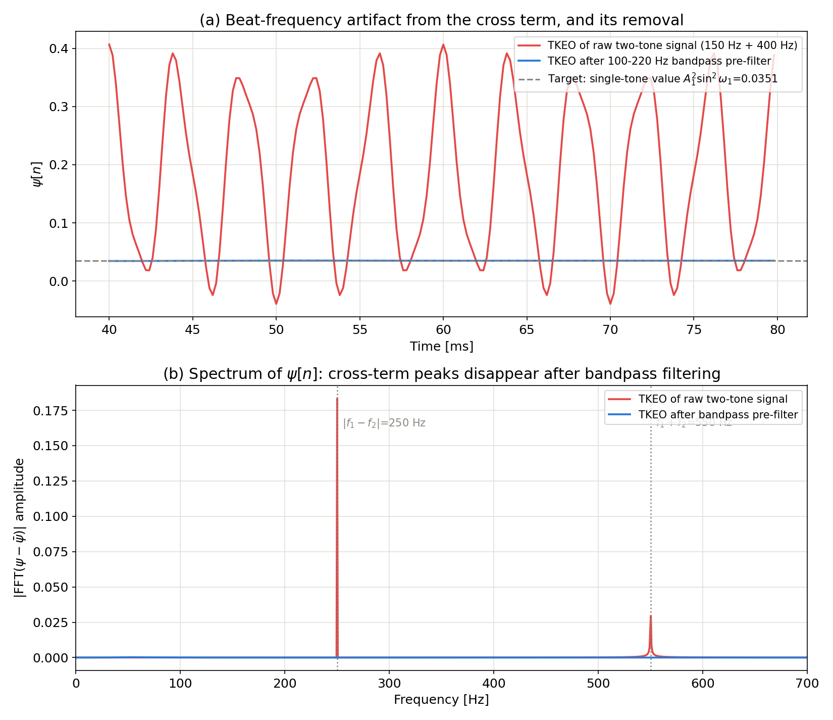
\[ c[n] = 2A_1A_2\left[\sin^2\!\left(\frac{\omega_1+\omega_2}{2}\right)\cos\big(\theta_1[n]-\theta_2[n]\big) + \sin^2\!\left(\frac{\omega_1-\omega_2}{2}\right)\cos\big(\theta_1[n]+\theta_2[n]\big)\right] \]\(\theta_1[n]-\theta_2[n]\) advances at angular frequency \(\omega_1-\omega_2\) , and \(\theta_1[n]+\theta_2[n]\) advances at angular frequency \(\omega_1+\omega_2\) . The cross term is therefore an exact sum of two pure sinusoids oscillating at the difference (beat) frequency \(\lvert f_1-f_2\rvert\) and the sum frequency \(f_1+f_2\) — frequencies present in neither \(\Psi[x_1][n]\) nor \(\Psi[x_2][n]\) (both constants, per the earlier derivation). This is the precise mathematical mechanism behind the well-known claim that “applying TKEO directly to a multi-component signal produces spurious instantaneous quantities.”
We verify this on a two-tone signal at 150 Hz and 400 Hz (amplitude ratio 0.8).
fs2 = 5000.0
f1, f2 = 150.0, 400.0
A1, A2 = 1.0, 0.8
w1, w2 = 2 * np.pi * f1 / fs2, 2 * np.pi * f2 / fs2
N2 = 8000
n2 = np.arange(N2)

x1 = A1 * np.cos(w1 * n2)
x2 = A2 * np.cos(w2 * n2)
psi1, psi2, psi12 = tkeo(x1), tkeo(x2), tkeo(x1 + x2)
cross = psi12 - psi1 - psi2
mid2 = slice(20, N2 - 20)


def fit_amplitude(sig, n_idx, freq_hz, fs):
    """Least-squares estimate of the amplitude of a given frequency component."""
    w = 2 * np.pi * freq_hz / fs
    design = np.column_stack([np.cos(w * n_idx), np.sin(w * n_idx)])
    coeffs, *_ = np.linalg.lstsq(design, sig, rcond=None)
    return np.hypot(coeffs[0], coeffs[1])


amp_diff = fit_amplitude(cross[mid2], n2[mid2], abs(f1 - f2), fs2)
amp_sum = fit_amplitude(cross[mid2], n2[mid2], f1 + f2, fs2)

print("psi1 mean:", psi1[mid2].mean(), " psi2 mean:", psi2[mid2].mean())
print("psi(x1+x2) mean:", psi12[mid2].mean(), " std:", psi12[mid2].std())
print("cross amplitude at |f1-f2|:", amp_diff, " at f1+f2:", amp_sum)
Results:
| Quantity | Theoretical | Measured |
|---|---|---|
| \(\Psi[x_1]\) (150 Hz alone, \(A_1^2\sin^2\omega_1\) ) | 0.035112 | 0.035112 |
| \(\Psi[x_2]\) (400 Hz alone, \(A_2^2\sin^2\omega_2\) ) | 0.148535 | 0.148535 |
| Cross-term amplitude @ \(\lvert f_1-f_2\rvert=250\) Hz | 0.183589 | 0.183556 |
| Cross-term amplitude @ \(f_1+f_2=550\) Hz | 0.039155 | 0.039000 |
For each pure tone alone, \(\Psi\) was perfectly constant (measured standard deviation essentially 0). Applying TKEO directly to the two-tone sum, \(\Psi[x_1+x_2][n]\) has a standard deviation of 0.132714 — and the amplitudes at 250 Hz and 550 Hz predicted by the closed form match the measured cross-term amplitudes to within 1% relative error. This is an artificial oscillation artifact that is the instantaneous energy of neither component.
The standard remedy: bandpass filtering before TKEO
The standard remedy used in the speech/biosignal onset-detection and DESA-based pitch/formant-tracking literature is to isolate the target component with a bandpass filter before applying TKEO. We apply a 100-220 Hz bandpass filter (4th-order Butterworth, zero-phase) to the two-tone signal above, isolating the 150 Hz component, before computing TKEO.
from scipy.signal import butter, filtfilt

b, a = butter(4, [100 / (fs2 / 2), 220 / (fs2 / 2)], btype="band")
x_bp = filtfilt(b, a, x1 + x2)
psi_bp = tkeo(x_bp)

print("raw std:", psi12[mid2].std(), " bandpass std:", psi_bp[mid2].std())
print("bandpass mean:", psi_bp[mid2].mean(), " target psi1:", psi1[mid2].mean())
Results: the standard deviation drops from 0.132714 (direct application) to 0.001223 after bandpass filtering — a ~108.5× reduction. The bandpass-filtered mean is 0.035124, closely matching the 150 Hz single-tone theoretical value of 0.035112. Excluding the 400 Hz component from the passband makes the beat/sum-frequency oscillation predicted by the closed-form cross term actually vanish, and the output converges to the single-component theoretical value — precisely why bandpass pre-filtering is nearly mandatory before TKEO in DESA-based pitch/formant tracking and bearing diagnostics.
Summary
- TKEO estimates a signal’s energy (proportional to amplitude² × frequency²) using only the 3-point product-sum \(\Psi[x[n]] = x[n]^2 - x[n-1]x[n+1]\) — an extremely lightweight nonlinear operator. A product-to-sum derivation shows this equals exactly \(A^2\sin^2\omega\) for a pure tone (reducing to \(A^2\omega^2\) under the narrowband approximation).
- The DESA-1 algorithm separates instantaneous amplitude and frequency from TKEO outputs; our numerical experiment showed it running ≈12× faster than the Hilbert transform with a practically sufficient 0.99999 amplitude correlation.
- Combined with a bandpass filter, TKEO alone (no EMD-family decomposition needed) correctly detected the bearing BPFO frequency (30.00 Hz, exactly matching ground truth).
- Noise sensitivity is analytically tractable: TKEO’s bias is exactly equal to the noise variance \(\sigma^2\) , independent of the signal — derived and verified numerically (relative error under 0.2%).
- The multi-component cross term also has a closed form, demonstrated to oscillate at the difference frequency \(\lvert f_1-f_2\rvert\) and sum frequency \(f_1+f_2\) ; bandpass pre-filtering suppresses its standard deviation by roughly 108×.
Related Articles
- https://yuhi-sa.github.io/en/posts/20260318_hilbert_transform/1/ — The other major approach to instantaneous amplitude/frequency estimation; prefer this when accuracy matters most
- https://yuhi-sa.github.io/en/posts/20260714_ceemdan_hht/1/ — The same bearing diagnostics task solved with CEEMDAN + Hilbert marginal spectrum
- https://yuhi-sa.github.io/en/posts/20260528_mode_decomposition/1/ — Fundamentals of EMD, VMD, and SSA mode decomposition
- https://yuhi-sa.github.io/en/posts/20260312_bandpass_filter/1/ — Bandpass filter design used as TKEO’s pre-processing step
- https://yuhi-sa.github.io/en/posts/20260524_time_frequency_guide/1/ — A hub article guiding the choice among time-frequency analysis methods
- https://yuhi-sa.github.io/en/posts/20260429_autocorrelation/1/ — Autocorrelation also smooths instantaneous quantities over a window; TKEO offers a sample-level-delay alternative for energy estimation
- https://yuhi-sa.github.io/en/posts/20260429_cepstrum/1/ — Another speech feature-extraction approach based on source-filter separation; a useful contrast with TKEO’s onset-detection angle
References
- Kaiser, J. F. (1990). “On a simple algorithm to calculate the ’energy’ of a signal.” ICASSP 1990.
- Maragos, P., Kaiser, J. F., & Quatieri, T. F. (1993). “Energy separation in signal modulations with application to speech analysis.” IEEE Transactions on Signal Processing, 41(10), 3024-3051.
- Ein Shoka, A. E., Dessouky, M. M., El-Sayed, A., & Hemdan, E. E. D. (2023). “An efficient CNN based epileptic seizures detection framework using encrypted EEG signals for secure telemedicine applications.” Alexandria Engineering Journal, 65, 399-412. (Uses TKEO to turn EEG into spectrograms for CNN-based seizure detection.)
- Bandela, S. R., Priyanka, S. S., Kumar, K. S., Reddy, Y. V. B., & Berhanu, A. A. (2023). “Stressed Speech Emotion Recognition Using Teager Energy and Spectral Feature Fusion with Feature Optimization.” Computational Intelligence and Neuroscience, 2023, 5765760.
- Chourdaki, I., Avramidis, K., Garoufis, C., Zlatintsi, A., & Maragos, P. (2025). “Teager-Kaiser Energy Methods for EEG Feature Extraction in Biomedical Applications.” arXiv:2511.17164. (Evaluates TKEO + Gabor filterbanks + energy separation across motor-imagery, emotion-recognition, and epilepsy-detection tasks.)
- scipy.signal.hilbert documentation