Introduction
https://yuhi-sa.github.io/en/posts/20260226_arima/1/ covered fitting ARMA/ARIMA models in Python with statsmodels.tsa.arima.model.ARIMA, noting in its related-articles section only that “https://yuhi-sa.github.io/en/posts/20260224_kalman_filter/1/ is a state-space estimation method, and comparing it to ARIMA is worthwhile” — without elaborating. In fact, statsmodels’ ARIMA estimation internally computes the exact Gaussian likelihood using a Kalman filter. This article converts an ARMA model into state-space form, derives the likelihood from the Kalman filter’s prediction-error decomposition, and implements maximum likelihood estimation from scratch. We then compare the result numerically against statsmodels and confirm the two agree to high precision.
State-Space Representation of ARMA Models (Harvey Form)
The ARMA(p, q) model
\[ x_t = \phi_1 x_{t-1} + \cdots + \phi_p x_{t-p} + \varepsilon_t + \theta_1 \varepsilon_{t-1} + \cdots + \theta_q \varepsilon_{t-q}, \qquad \varepsilon_t \sim \mathcal{N}(0, \sigma^2) \tag{1} \]can be rewritten as a state-space model in companion form using an \(m = \max(p, q+1)\) -dimensional state vector (Harvey, 1993):
\[ \boldsymbol{\alpha}_{t} = T \boldsymbol{\alpha}_{t-1} + R \varepsilon_{t}, \qquad y_t = Z \boldsymbol{\alpha}_t \tag{2} \]For ARMA(1,1) (\(m = \max(1, 2) = 2\) ), this becomes concretely
\[ T = \begin{bmatrix} \phi & 1 \\ 0 & 0 \end{bmatrix}, \qquad R = \begin{bmatrix} 1 \\ \theta \end{bmatrix}, \qquad Z = \begin{bmatrix} 1 & 0 \end{bmatrix} \tag{3} \]The state’s first component is \(\alpha_t^{(1)} = x_t\) and the second is \(\alpha_t^{(2)} = \theta \varepsilon_t\) . Expanding equations (2)-(3) directly gives
\[ \alpha_t^{(1)} = \phi \alpha_{t-1}^{(1)} + \alpha_{t-1}^{(2)} + \varepsilon_t = \phi x_{t-1} + \theta \varepsilon_{t-1} + \varepsilon_t \tag{4} \]which matches the ARMA(1,1) equation (1) exactly. Mapping onto the notation from https://yuhi-sa.github.io/en/posts/20260224_kalman_filter/1/: transition matrix \(A=T\) , observation matrix \(H=Z\) , process-noise covariance \(Q = R R^\top \sigma^2\) (rank 1), and observation noise \(R_{\text{obs}} = 0\) (the observation is exactly a linear combination of the state, with no additional measurement error) — a special case of the general Kalman-filter setup.
The Stationary Initial Distribution: A Discrete Lyapunov Equation
If the ARMA model is stationary (e.g., \(|\phi| < 1\) ), the state vector’s unconditional mean is \(\mathbf{0}\) , and its unconditional covariance \(P_0\) solves the discrete Lyapunov equation
\[ P_0 = T P_0 T^\top + R R^\top \sigma^2 \tag{5} \]Solving this matrix equation directly with scipy.linalg.solve_discrete_lyapunov gives the Kalman filter its correct initial covariance (initializing with a zero matrix or a large arbitrary value distorts the likelihood during the burn-in period before convergence — we quantify this empirically in the numerical experiment below).
Caveat: The Lyapunov Equation Breaks Down Near Non-Stationarity
The \(P_0\)
returned by solve_discrete_lyapunov is only meaningful when the stationarity condition \(|\phi| < 1\)
holds. To see how fragile this boundary is, fix \(\theta=0.4\)
, \(\sigma^2=1\)
and push \(\phi\)
toward the unit circle:
| \(\phi\) | solve_discrete_lyapunov result \(P_0[0,0]\) | Note |
|---|---|---|
| 0.99 | 98.09 | Stationary but close to the unit root; variance explodes |
| 1.00 | (exception) | LinAlgError: A singular matrix detected |
| 1.01 | -97.91 | Non-stationary, yet no exception — a negative “variance” |
At \(\phi=1.01\)
(an explosive process), solve_discrete_lyapunov raises no exception at all — it silently returns a matrix with a negative diagonal entry, which is not a valid covariance matrix. Fortunately, feeding this value straight into the Kalman filter makes the first-step predictive variance negative with the same sign (empirically, \(F_1 = -97.91\)
— the same magnitude as the large positive value at \(\phi=0.99\)
, just flipped). The if F <= 0: return 1e10 guard in the Python implementation below is not merely generic numerical hygiene — it specifically catches the case where an optimizer such as Nelder-Mead wanders into the non-stationary region and penalizes the objective function heavily to push it back out. Reparameterizing \(\phi\)
to stay in \((-1, 1)\)
(e.g., \(\phi = \tanh(u)\)
) would exclude this region from the search space entirely.
Note also that for ARIMA(\(p, d, q\)
) models with \(d > 0\)
, even though the differenced ARMA part is stationary, a formulation that keeps the pre-differenced series in the state vector carries the unit-root component directly in the state, so the stationary covariance in equation (5) does not exist. In practice, such non-stationary components are initialized with a “diffuse prior” — formally infinite variance — and its influence is excluded from the likelihood once the filter has converged (this is what R’s stats::arima and the exact diffuse initialization in the KFAS package do). This article does not go into that extension and focuses on the stationary ARMA case (\(d=0\)
).
Exact Log-Likelihood via the Kalman Filter
Applying the Kalman filter to state-space model (2) produces, at each time step, the prediction error (innovation) \(e_t = y_t - Z\boldsymbol{\alpha}_{t|t-1}\) and its variance \(F_t = Z P_{t|t-1} Z^\top\) . Under the Gaussian assumption, the joint density of the observations factors via the prediction error decomposition as
\[ \log L(\boldsymbol{\theta}) = -\frac{1}{2}\sum_{t=1}^{N}\left[\log(2\pi F_t) + \frac{e_t^2}{F_t}\right] \tag{6} \]This is the exact (not approximate) Gaussian log-likelihood for the ARMA/ARIMA model, and it’s what statsmodels and most other statistical software compute via the Kalman filter under the hood. Numerically maximizing (6) over \(\boldsymbol{\theta} = (\phi, \theta, \sigma^2)\) yields the maximum likelihood estimate.
Caveat: Degeneracy When Observation Noise Is Exactly Zero
The ARMA state-space representation in equation (3) has no measurement error (\(R_{\text{obs}}=0\) ). As a result, the \((1,1)\) entry of the updated state covariance \(P_{t\vert t}\) — the variance of the state component corresponding to \(y_t\) — collapses to exactly \(0\) , both theoretically and numerically. Running the Kalman filter with the fitted parameters below (\(\hat\phi=0.676518\) , \(\hat\theta=0.420873\) , \(\hat\sigma^2=0.959929\) ) confirms this:
| \(t\) | \(P_{t\vert t}[0,0]\) | \(\hat\alpha_{t\vert t}^{(1)}\) (updated state) | \(y_t\) (observation) |
|---|---|---|---|
| 0 | 0.0 | 0.4967141530 | 0.4967141530 |
| 1 | 0.0 | 0.4081212671 | 0.4081212671 |
| 2 | 0.0 | 0.8780677046 | 0.8780677046 |
The updated filter state matches the observation \(y_t\) exactly (to the digits shown). This is unsurprising — the observation reveals the first state component with no error at all. It might look like “the filter isn’t doing anything,” but the information actually flows through the prediction before the update, \(a_{t\vert t-1}\) and its variance \(F_{t\vert t-1}\) — these are exactly what build up the likelihood in equation (6) and the prediction interval in the figure below. Looking only at the “post-update” values of the Kalman filter gives a trivial result for this particular model.
Python Implementation
import numpy as np
from scipy.optimize import minimize
from scipy.linalg import solve_discrete_lyapunov

def kf_loglik(params, y):
    phi, theta, log_sigma2 = params
    sigma2 = np.exp(log_sigma2)
    T = np.array([[phi, 1.0], [0.0, 0.0]])
    R = np.array([1.0, theta])
    Z = np.array([1.0, 0.0])
    Q = np.outer(R, R) * sigma2

    P = solve_discrete_lyapunov(T, Q)  # stationary initial covariance
    a = np.zeros(2)

    ll = 0.0
    for t in range(len(y)):
        a_pred = T @ a
        P_pred = T @ P @ T.T + Q
        F = Z @ P_pred @ Z.T
        if F <= 0:
            return 1e10
        e = y[t] - Z @ a_pred
        ll += -0.5 * (np.log(2 * np.pi * F) + e**2 / F)
        K = P_pred @ Z.T / F          # Kalman gain
        a = a_pred + K * e
        P = P_pred - np.outer(K, Z @ P_pred)
    return -ll  # negate for minimization

# MLE, starting from phi=0, theta=0, log(sigma^2)=0
x0 = np.array([0.0, 0.0, 0.0])
res = minimize(kf_loglik, x0, args=(x,), method="Nelder-Mead",
               options={"xatol": 1e-8, "fatol": 1e-8, "maxiter": 5000})
phi_hat, theta_hat, sigma2_hat = res.x[0], res.x[1], np.exp(res.x[2])
solve_discrete_lyapunov(T, Q) solves equation (5) for the stationary initial covariance \(P_0\)
; K = P_pred @ Z.T / F inside the loop is the Kalman gain, and ll += ... accumulates the log-likelihood from equation (6).
Numerical Experiment: Agreement with statsmodels
We simulated 500 samples of an ARMA(1,1) process with true parameters \(\phi=0.7\)
, \(\theta=0.4\)
, \(\sigma^2=1.0\)
using statsmodels.tsa.arima_process.ArmaProcess (with np.random.seed(42) fixed for reproducibility), then fit both the from-scratch KF-MLE above and statsmodels.tsa.arima.model.ARIMA(order=(1,0,1)) to the same data.
Caveat: Watch Out for ARIMA’s Default Constant Term
statsmodels’ ARIMA(y, order=(1,0,1)) fits a constant term by default (trend="c"). Since our state-space representation (2)-(3) assumes a zero-mean ARMA process, comparing against the default-fitted model leaves a small but nonzero constant (empirically about \(0.035\)
) unaccounted for, which throws off the likelihood comparison — on the author’s first run this produced a log-likelihood discrepancy of \(1.7 \times 10^{-2}\)
, which took some digging to track down. To compare against the correct zero-mean model, trend="n" must be set explicitly.
fit = ARIMA(x, order=(1, 0, 1), trend="n").fit()
The results below are all computed with trend="n".
| Parameter | From-scratch KF | statsmodels | Difference |
|---|---|---|---|
| \(\phi\) | 0.676518 | 0.676520 | 1.8×10⁻⁶ |
| \(\theta\) | 0.420873 | 0.420870 | 2.5×10⁻⁶ |
| \(\sigma^2\) | 0.959929 | 0.959929 | 1.2×10⁻⁷ |
| Log-likelihood | -699.899146 | -699.899146 | 1.2×10⁻⁹ |
Parameter estimates and log-likelihood agree to six or more decimal places. The residual differences are numerical-optimization noise from Nelder-Mead vs. statsmodels’ internal optimizer — both are maximizing the same objective function. Both estimates deviate noticeably from the true values (\(\phi=0.7\) , \(\theta=0.4\) ), which is ordinary finite-sample estimation error at \(N=500\) (statsmodels reports standard errors of \(0.0392\) for \(\phi\) and \(0.0492\) for \(\theta\) ).
We also compared 5-step-ahead forecasts computed from the fitted filtered state against fit.forecast(5): the maximum absolute difference was \(5.8 \times 10^{-6}\)
. Likelihood, parameters, and forecasts all agree, numerically confirming that the state-space representation and Kalman filter are the correct computational foundation for ARIMA estimation.
Figure: One-Step-Ahead Prediction and the Effect of the \(P_0\) Choice on Likelihood
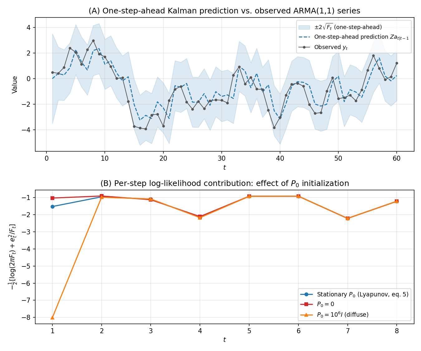
Panel (A) above overlays the one-step-ahead prediction \(Z a_{t\vert t-1}\) and its prediction interval \(\pm 2\sqrt{F_{t\vert t-1}}\) , computed with the fitted parameters, on the observed series. The predictive standard deviation converges to \(\sqrt{F_\infty} \approx 0.980\) in steady state, but is slightly wider at \(t=1\) (\(\sqrt{F_1} \approx 1.758\) ) — the very first prediction, which still uses the raw initial covariance \(P_0\) — before quickly settling to its steady-state value.
Panel (B) puts numbers behind the claim made earlier in this article that “initializing with a zero matrix or a large arbitrary value distorts the likelihood.” The total log-likelihood computed with the three initializations is \(-699.899146\) for the Lyapunov-equation solution (this article’s method), \(-699.343158\) for zero initialization, and \(-706.422969\) for the diffuse prior (\(10^6 I\) ) — a difference of up to about \(6.5\) . Looking at just \(t=1\) , the gap is even more striking: the per-step log-likelihood terms are \(-1.523\) (Lyapunov), \(-1.027\) (zero), and \(-8.015\) (diffuse), but by \(t=2\) all three have converged to nearly the same value (the Kalman filter “forgets” the effect of a wrong initial value as observations accumulate). The smaller the sample size, the more this initialization error can distort the likelihood and parameter estimates, which is why the exact stationary initialization via equation (5) is recommended for stationary ARMA models.
Why This Understanding Matters in Practice
- Handling missing observations: The Kalman filter naturally skips the update step at any time index with a missing observation. This is exactly why statsmodels’ ARIMA can fit a series with missing values without any special preprocessing.
- Generalizing to state-space models: Introducing observation noise \(R_{\text{obs}} > 0\) immediately extends the model to “ARMA signal plus measurement noise.” This directly demonstrates that ARIMA is a special case of the general state-space model covered in https://yuhi-sa.github.io/en/posts/20260224_kalman_filter/1/.
- Extending to time-varying parameters: Just as https://yuhi-sa.github.io/en/posts/20260715_rls_adaptive_filter/1/ showed RLS is a special case of the Kalman filter, allowing the ARMA coefficients to vary over time (time-varying AR models, state-space TVP-VAR) fits naturally into the same Kalman-filter framework.
- Generalizing to multiple series: This article covers univariate ARMA, but the same state-space representation and Kalman-filter maximum likelihood estimation extends directly to multivariate VARMA models. A 2024 review of VARMA models by Düker et al. lists “state-space representations and the Kalman filter” as one of the primary estimation approaches in its discussion of identification, estimation, and diagnostics — confirming that the argument in this article is not limited to the univariate special case.
Related Articles
- ARIMA and SARIMA: Theory and Python Implementation - The foundation for fitting ARIMA models in statsmodels. This article explains the estimation machinery working underneath it.
- GARCH(1,1) in Python - A companion article using the same prediction-error-decomposition framework to model conditional variance instead of the mean.
- Kalman Filter: Theory and Python Implementation - The state-space model and Kalman filter notation used throughout this article.
- The RLS Algorithm in Python: Recursive Least Squares and Its Equivalence to the Kalman Filter - A companion article deriving adaptive filtering as another special case of the Kalman filter.
- PACF and AR Order Identification - Methods for choosing the AR order \(p\) , directly relevant to sizing the state dimension \(m\) here.
- Time Series Anomaly Detection: From Statistical Methods to Kalman Filters - An application of state-space models to anomaly detection.
- Autocorrelation Function: Theory and Python Implementation - Useful background on the theoretical autocorrelation structure of ARMA models.
- Choosing Among Time-Series Methods: Forecasting, Classification, and Anomaly Detection - A selection guide across seven methods including ARIMA and Kalman filters.
References
- Harvey, A. C. (1993). Time Series Models (2nd ed.). MIT Press. Chapter 3 (State space form of ARMA models).
- Hamilton, J. D. (1994). Time Series Analysis. Princeton University Press. Chapter 13 (The Kalman Filter).
- Durbin, J., & Koopman, S. J. (2012). Time Series Analysis by State Space Methods (2nd ed.). Oxford University Press.
- Seabold, S., & Perktold, J. (2010). statsmodels: Econometric and statistical modeling with python. Proceedings of the 9th Python in Science Conference.
- Düker, M.-C., Matteson, D. S., Tsay, R. S., & Wilms, I. (2024). Vector Autoregressive Moving Average Models: A Review. arXiv:2406.19702.