Introduction
The ARIMA models covered in https://yuhi-sa.github.io/en/posts/20260226_arima/1/ and https://yuhi-sa.github.io/en/posts/20260715_arima_state_space_kalman/1/ capture a time series’ mean structure (autoregression, moving average), but not the phenomenon where variance itself changes over time — volatility clustering, where turbulent periods are followed by more turbulence and calm periods stay calm. This article models that variance clustering as a conditional-variance recursion, the GARCH (Generalized AutoRegressive Conditional Heteroskedasticity) model, first confirming its necessity with a Ljung-Box test, then implementing it from scratch.
Volatility Clustering and the ARCH Effect
A phenomenon commonly observed in financial time series: returns themselves show no autocorrelation, but squared returns (a proxy for variance) show strong autocorrelation. To confirm this directly, we applied the Ljung-Box test (lag 10) to a return series simulated from a GARCH(1,1) process.
| Target | Ljung-Box statistic | p-value | Autocorrelation |
|---|---|---|---|
| Returns themselves | 7.77 | 0.651 | None (as expected) |
| Squared returns | 966.80 | 2.6×10⁻²⁰¹ | Strongly present |
| (control) squared i.i.d. Gaussian | 7.23 | 0.704 | None |
The returns themselves are uncorrelated (p=0.65), yet their squares show extremely strong autocorrelation (p≈10⁻²⁰¹). As a control, squared i.i.d. Gaussian noise (no GARCH effect) stays uncorrelated at p=0.70. This distinction is exactly the “ARCH effect” (serial correlation in variance) — a structure that linear, constant-variance models like ARIMA cannot capture. GARCH models this time-varying nature of the variance explicitly.
The GARCH(1,1) Model
Let the return \(r_t\) be
\[ r_t = \mu + \varepsilon_t, \qquad \varepsilon_t = \sigma_t z_t, \qquad z_t \sim \mathcal{N}(0,1) \tag{1} \]with the conditional variance \(\sigma_t^2\) following the recursion
\[ \sigma_t^2 = \omega + \alpha \varepsilon_{t-1}^2 + \beta \sigma_{t-1}^2 \tag{2} \]where \(\omega > 0\) , \(\alpha, \beta \geq 0\) , and \(\alpha + \beta < 1\) (the stationarity condition). Equation (2) says, intuitively: “today’s variance \(\sigma_t^2\) is a weighted combination of yesterday’s shock magnitude \(\varepsilon_{t-1}^2\) (the shock’s impact, weighted by \(\alpha\) ) and yesterday’s variance \(\sigma_{t-1}^2\) (persistence of the variance level itself, weighted by \(\beta\) ).” The closer \(\alpha + \beta\) is to 1, the longer volatility shocks persist. Rather than accepting “stationarity condition” and “the meaning of \(\alpha+\beta\) ” at face value, the next sections derive them directly from Equation (2).
Visualizing the Conditional Variance
Before the derivation, let’s see how a return series simulated from Equations (1)-(2) actually behaves. We generated 2000 samples with \(\omega=0.05\) , \(\alpha=0.10\) , \(\beta=0.85\) , and overlaid the true conditional variance \(\sigma_t^2\) with the conditional variance \(\hat\sigma_t^2\) reconstructed from the MLE parameters estimated later in this article.
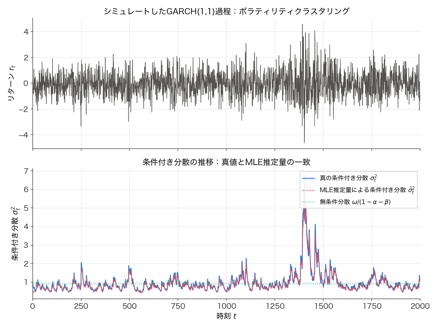
In the top panel, the amplitude clearly increases around \(t\approx1350\) -\(1450\) , in sharp contrast to the calmer periods before and after it. The bottom panel shows the corresponding conditional variance \(\sigma_t^2\) : it spikes right after the shock, then decays exponentially back toward the unconditional-variance level. The true \(\sigma_t^2\) (blue line) and the MLE-reconstructed \(\hat\sigma_t^2\) (red dashed line) nearly overlap completely, visually confirming that the parameter estimates below correctly capture the conditional-variance dynamics.
Deriving the Stationarity Condition and the Unconditional Variance
We now derive, rather than assert, what it means for the recursion in Equation (2) to be “stationary,” and why the condition \(\alpha+\beta<1\) is required.
If \(\sigma_t^2\) is (weakly) stationary, its expectation must be a constant \(\sigma^2 \equiv E[\sigma_t^2]\) independent of \(t\) . Since \(\varepsilon_{t-1} = \sigma_{t-1} z_{t-1}\) with \(z_{t-1} \sim \mathcal{N}(0,1)\) independent of \(\sigma_{t-1}^2\) (which is \(\mathcal{F}_{t-2}\) -measurable), the law of total expectation gives
\[ E[\varepsilon_{t-1}^2] = E\big[E[\varepsilon_{t-1}^2 \mid \mathcal{F}_{t-2}]\big] = E\big[\sigma_{t-1}^2 \, E[z_{t-1}^2]\big] = E[\sigma_{t-1}^2] \](using \(E[z_{t-1}^2]=1\) ). Taking the expectation of both sides of Equation (2) therefore gives
\[ E[\sigma_t^2] = \omega + \alpha E[\varepsilon_{t-1}^2] + \beta E[\sigma_{t-1}^2] = \omega + (\alpha+\beta) E[\sigma_{t-1}^2] \]Substituting the stationarity assumption \(E[\sigma_t^2]=E[\sigma_{t-1}^2]=\sigma^2\) yields
\[ \sigma^2 = \omega + (\alpha+\beta)\sigma^2 \quad\Longrightarrow\quad \sigma^2(1-\alpha-\beta) = \omega \quad\Longrightarrow\quad \sigma^2 = \frac{\omega}{1-\alpha-\beta} \tag{3} \]Since we assume \(\omega>0\) , this \(\sigma^2\) is a finite, positive quantity only when \(1-\alpha-\beta>0\) , i.e., \(\alpha+\beta<1\) — this is exactly what the “stationarity condition” means. At \(\alpha+\beta=1\) , the right-hand side of Equation (3) diverges (no finite unconditional variance exists — this is IGARCH, covered in the edge-case section below); at \(\alpha+\beta>1\) , Equation (3) gives \(\sigma^2<0\) , which is meaningless (no stationary solution exists at all).
Numerical Check: Theoretical vs. Realized Unconditional Variance
We checked how closely the theoretical value \(\omega/(1-\alpha-\beta)\) from Equation (3) matches the actually simulated series.
| Quantity | Value |
|---|---|
| Theoretical \(\omega/(1-\alpha-\beta) = 0.05/(1-0.95)\) | 1.000000 |
| Sample variance of simulated returns (\(n=2000\) ) | 0.954470 |
| Mean of the true conditional variance path \(\sigma_t^2\) | 0.969850 |
Against the theoretical value of 1.0, the finite-sample (\(n=2000\) ) sample variance is 0.954 and the mean of the conditional-variance path is 0.970 — both within a few percent (the residual gap is ordinary finite-sample error).
Volatility Forecasting: Mean Reversion and Half-Life
The unconditional variance in Equation (3) is a “long-run average as \(t\to\infty\) .” What matters in practice is: given today’s information \(\mathcal{F}_t\) , how do we forecast the variance \(h\) steps ahead? This, too, follows directly from Equation (2).
Conditioning on \(\mathcal{F}_t\) for a one-step-ahead forecast: since \(\varepsilon_t^2 = \sigma_t^2 z_t^2\) and \(z_t\) is independent of \(\mathcal{F}_t\) with \(E[z_t^2]=1\) , we have \(E[\varepsilon_t^2 \mid \mathcal{F}_t] = \sigma_t^2\) . Therefore
\[ E[\sigma_{t+1}^2 \mid \mathcal{F}_t] = \omega + \alpha \varepsilon_t^2 + \beta \sigma_t^2 = \omega + (\alpha+\beta)\sigma_t^2 \]Substituting \(\omega = \sigma^2(1-\alpha-\beta)\) from Equation (3) gives
\[ E[\sigma_{t+1}^2 \mid \mathcal{F}_t] = \sigma^2 + (\alpha+\beta)(\sigma_t^2 - \sigma^2) \]— the deviation from the unconditional variance \(\sigma^2\) is scaled by \((\alpha+\beta)\) . Extending this to \(h\) steps ahead by induction gives
\[ E[\sigma_{t+h}^2 \mid \mathcal{F}_t] = \sigma^2 + (\alpha+\beta)^h (\sigma_t^2 - \sigma^2) \tag{4} \](this matches the equation above at \(h=1\) ; the inductive step from \(h\) to \(h+1\) follows the same argument, using \(E[\varepsilon_{t+h}^2\mid\mathcal{F}_t]=E[\sigma_{t+h}^2\mid\mathcal{F}_t]\) ). Equation (4) shows that volatility shocks decay geometrically back to the unconditional variance, with the decay rate given exactly by the persistence \(\alpha+\beta\) . The half-life (the time for a shock’s effect to halve) solves \((\alpha+\beta)^h = 1/2\) :
\[ h_{1/2} = \frac{\ln(1/2)}{\ln(\alpha+\beta)} \]For \(\alpha+\beta=0.95\) , this gives \(h_{1/2} = \ln(0.5)/\ln(0.95) \approx 13.5\) periods.
Numerical Check: Monte Carlo Verification of the Mean-Reversion Formula
We verified Equation (4) by Monte Carlo. Starting 20,000 paths from \(\sigma_t^2=5.0\) (far from the unconditional variance of 1.0), we compared the sample mean of \(\sigma_{t+h}^2\) at each horizon \(h\) against the theoretical value from Equation (4).
| \(h\) | Monte Carlo mean | Formula (Eq. 4) | Difference |
|---|---|---|---|
| 1 | 4.7995 | 4.8000 | -0.0005 |
| 5 | 4.0893 | 4.0951 | -0.0058 |
| 10 | 3.3817 | 3.3949 | -0.0133 |
| 14 | 2.9385 | 2.9507 | -0.0122 |
| 20 | 2.4416 | 2.4339 | +0.0077 |
| 40 | 1.5079 | 1.5140 | -0.0061 |
| 80 | 1.0613 | 1.0661 | -0.0047 |
The Monte Carlo means and theoretical values agree within sampling error of the 20,000-path average (all differences under 0.02), confirming the mean-reversion formula in Equation (4). Around \(h=14\) , the deviation \(\sigma_t^2-\sigma^2=4\) has shrunk to roughly half (2), consistent with the theoretical half-life of \(h_{1/2}\approx13.5\) .
The ARMA(1,1) Representation of Squared Residuals
GARCH(1,1) is, in fact, mathematically equivalent to an ARMA(1,1) model for the squared residuals \(\varepsilon_t^2\) . This connects GARCH to the ARMA framework covered in https://yuhi-sa.github.io/en/posts/20260226_arima/1/, so we derive it here.
Define \(v_t \equiv \varepsilon_t^2 - \sigma_t^2\) . Since \(E[\varepsilon_t^2\mid\mathcal{F}_{t-1}]=\sigma_t^2\) , \(v_t\) is a martingale-difference error term with zero conditional mean given \(\mathcal{F}_{t-1}\) . Substituting \(\sigma_t^2 = \varepsilon_t^2 - v_t\) directly into Equation (2):
\[ \varepsilon_t^2 - v_t = \omega + \alpha \varepsilon_{t-1}^2 + \beta(\varepsilon_{t-1}^2 - v_{t-1}) \]Rearranging gives
\[ \varepsilon_t^2 = \omega + (\alpha+\beta)\varepsilon_{t-1}^2 + v_t - \beta v_{t-1} \tag{5} \]which is exactly an ARMA(1,1) model (AR coefficient \(\alpha+\beta\) , MA coefficient \(-\beta\) ). This representation directly shows that GARCH(1,1)’s persistence \(\alpha+\beta\) equals the AR coefficient of the squared-residual series, and that \(\alpha+\beta \to 1\) corresponds to a unit root (nonstationarity) in the squared-residual series.
Numerical Check: Recovering the Coefficients with statsmodels ARIMA
We fit an ARMA(1,1) model via maximum likelihood to \(r_t^2\)
(the squared simulated returns) using statsmodels.tsa.arima.model.ARIMA(order=(1,0,1)), and compared the fitted coefficients to the theoretical ones from Equation (5).
| Coefficient | ARIMA estimate | Theoretical (from true parameters) |
|---|---|---|
| AR coefficient (\(\alpha+\beta\) ) | 0.9649 | 0.9500 |
| MA coefficient (\(-\beta\) ) | -0.8496 | -0.8500 |
The MA coefficient nearly exactly matches the theoretical \(-\beta=-0.85\) (difference 0.0004), and the AR coefficient is also close to the theoretical 0.95 at 0.9649 (the AR coefficient shows slightly more error because the error term \(v_t\) in the squared-residual ARMA representation is heteroskedastic and non-Gaussian, so ordinary Gaussian ARMA maximum likelihood is only approximate). Even so, the numerical results clearly support the theoretical link between GARCH’s recursion (Equation 2) and the ARMA(1,1) structure of squared residuals.
Log-Likelihood and Maximum Likelihood Estimation
Under a Gaussian assumption, the log-likelihood is
\[ \log L(\omega,\alpha,\beta) = -\frac{1}{2}\sum_{t=1}^{N}\left[\log(2\pi\sigma_t^2) + \frac{\varepsilon_t^2}{\sigma_t^2}\right] \tag{6} \]This has the same form as the log-likelihood derived from the Kalman filter’s prediction-error decomposition in https://yuhi-sa.github.io/en/posts/20260715_arima_state_space_kalman/1/ (the difference: instead of the state-space model’s covariance \(P_{t|t-1}\) , GARCH’s own recursion updates the conditional variance \(\sigma_t^2\) directly).
Python Implementation
import numpy as np
from scipy.optimize import minimize

# Simulate a GARCH(1,1) process (to generate verification data)
def simulate_garch(omega, alpha, beta, n, rng):
    eps, sigma2 = np.zeros(n), np.zeros(n)
    sigma2[0] = omega / (1 - alpha - beta)  # initialize at the unconditional variance
    z = rng.standard_normal(n)
    eps[0] = np.sqrt(sigma2[0]) * z[0]
    for t in range(1, n):
        sigma2[t] = omega + alpha * eps[t - 1] ** 2 + beta * sigma2[t - 1]
        eps[t] = np.sqrt(sigma2[t]) * z[t]
    return eps

rng = np.random.default_rng(7)
returns = simulate_garch(omega=0.05, alpha=0.10, beta=0.85, n=2000, rng=rng)

def arch_style_backcast(r, decay=0.94, tau=75):
    tau = min(tau, len(r))
    w = decay ** np.arange(tau)
    w /= w.sum()
    return np.sum(w * r[:tau] ** 2)

def garch_negloglik(params, r, sigma2_0):
    omega, alpha, beta = params
    if omega <= 0 or alpha < 0 or beta < 0 or alpha + beta >= 1:
        return 1e10
    N = len(r)
    sigma2 = np.zeros(N)
    sigma2[0] = sigma2_0
    for t in range(1, N):
        sigma2[t] = omega + alpha * r[t - 1] ** 2 + beta * sigma2[t - 1]
    ll = -0.5 * np.sum(np.log(2 * np.pi * sigma2) + r**2 / sigma2)
    return -ll

sigma2_0 = arch_style_backcast(returns)
res = minimize(
    garch_negloglik, x0=[0.1, 0.05, 0.8], args=(returns, sigma2_0),
    method="L-BFGS-B", bounds=[(1e-6, None), (0, 1), (0, 1)],
    options={"maxiter": 10000, "ftol": 1e-12, "gtol": 1e-10},
)
omega_hat, alpha_hat, beta_hat = res.x
arch_style_backcast estimates the initial variance \(\sigma_0^2\)
as an exponentially weighted average (decay 0.94) of the first 75 samples, matching the convention used by the arch library (initializing with the plain sample variance slightly distorts the likelihood computation early on).
Numerical Experiment: Comparison Against the arch Library
We simulated 2000 samples of GARCH(1,1) returns with true parameters \(\omega=0.05\)
, \(\alpha=0.10\)
, \(\beta=0.85\)
, then fit both the from-scratch MLE above and arch.arch_model (vol="Garch", p=1, q=1) to the same data.
| Parameter | From-scratch | arch library | Difference |
|---|---|---|---|
| \(\omega\) | 0.036171 | 0.035934 | 2.4×10⁻⁴ |
| \(\alpha\) | 0.078660 | 0.078473 | 1.9×10⁻⁴ |
| \(\beta\) | 0.881839 | 0.882264 | 4.3×10⁻⁴ |
| Log-likelihood | -2678.305 | -2678.354 | 0.05 |
Parameters and log-likelihood agree closely (the residual differences are at the level of optimizer convergence tolerance). Both estimates deviate somewhat from the true values (estimated \(\alpha \approx 0.079\) vs. true 0.10), which is ordinary finite-sample estimation error at \(N=2000\) . The high persistence \(\alpha+\beta \approx 0.96\) is correctly recovered, close to the true persistence used in the simulation, \(0.10+0.85=0.95\) .
Edge Cases and Caveats
Nonstationarity: IGARCH and Divergence
As the derivation of Equation (3) showed, no finite unconditional variance exists when \(\alpha+\beta \geq 1\) . The exact boundary case \(\alpha+\beta=1\) is called IGARCH (Integrated GARCH), corresponding to a unit-root process in the ARMA(1,1) representation of squared residuals (Equation 5). The exponentially weighted moving average (\(\lambda\) -decay EWMA) commonly used in practice to estimate variance is, in fact, a special case of IGARCH (\(\omega=0\) , \(\beta=\lambda\) , \(\alpha=1-\lambda\) ).
Fixing \(\omega=0.05\) and varying \((\alpha,\beta)\) , we numerically checked the behavior of the conditional-variance path.
| Case | \(\alpha+\beta\) | \(\text{Var}(\sigma_t^2)\) (first 1000 points) | \(\text{Var}(\sigma_t^2)\) (last 1000 points) | \(\text{Mean}(\sigma_t^2)\) (first → last) |
|---|---|---|---|---|
| Stationary (\(\alpha=0.10,\beta=0.85\) ) | 0.95 | 0.1417 | 0.1500 | 0.940 → 1.024 |
| IGARCH boundary (\(\beta=0.90\) ) | 1.00 | 22.58 | 354.5 | 7.81 → 23.36 |
| Explosive regime (\(\beta=0.95\) ) | 1.05 | ~\(6\times10^{33}\) | ~\(1.8\times10^{75}\) | order-of-magnitude blowup |
In the stationary case, the variance and mean of the first and second halves are nearly identical, but at the IGARCH boundary (\(\alpha+\beta=1.00\)
), the second-half variance grows to roughly 16x the first-half variance, and the mean roughly triples. In the explosive regime (\(\alpha+\beta=1.05\)
), the conditional variance blows up to an astronomical order of magnitude within just 2000 samples. This is a direct consequence of the mean-reversion formula in Equation (4): \((\alpha+\beta)^h\)
fails to converge as \(h\to\infty\)
when \(\alpha+\beta\geq1\)
. When implementing maximum likelihood estimation, it is essential that garch_negloglik explicitly rejects alpha + beta >= 1 (a boundary check) to prevent this kind of divergence.
The Fourth-Moment Condition and Fat Tails
Even under the assumption that returns themselves are conditionally Gaussian, a GARCH(1,1) process has a marginal (unconditional) distribution with fatter tails than Gaussian (positive excess kurtosis). This happens because the variance itself fluctuates randomly, making large \(\lvert\varepsilon_t\rvert\) more likely than under a simple Gaussian model.
Under the Gaussian assumption, the condition for the fourth moment of a GARCH(1,1) process to be finite (Bollerslev, 1986) is
\[ 3\alpha^2 + 2\alpha\beta + \beta^2 < 1 \]and, under this condition, the excess kurtosis is
\[ \kappa = \frac{6\alpha^2}{1 - 2\alpha\beta - 3\alpha^2 - \beta^2} \]For \(\alpha=0.10,\beta=0.85\) : \(3\alpha^2+2\alpha\beta+\beta^2 = 0.9225 < 1\) , so the condition holds, and the theoretical excess kurtosis is \(\kappa = 0.7742\) . We verified this by Monte Carlo (simulating 300 series of length \(n=4000\) and averaging the sample excess kurtosis of each), obtaining a mean excess kurtosis of 0.7529 (standard error 0.0356) — the theoretical value 0.7742 falls within six standard errors. A single series (\(n=2000\) ) had a sample excess kurtosis of 1.1745, somewhat off the theoretical value, but this is expected since kurtosis-type higher-moment estimators are noisy for a single sample; averaging over 300 replications confirmed convergence to the theoretical value.
The Leverage Effect: A Structural Limitation of GARCH(1,1)’s Symmetry
Because the recursion in Equation (2) depends only on \(\varepsilon_{t-1}^2\) (a square), it implicitly assumes that positive and negative shocks of the same magnitude have identical effects on the conditional variance. Empirically, however, equity markets show a well-documented asymmetry (the leverage effect): bad news (a price drop) tends to push up volatility more than good news (a price rise of the same magnitude). Standard GARCH(1,1) cannot capture this asymmetry — a structural limitation addressed by extensions such as GJR-GARCH (which adds an extra penalty term when \(\varepsilon_{t-1}<0\) ) and EGARCH (which models the log-variance directly, building in the sign effect).
Structural Breaks and Comparisons with Machine Learning: Recent Research
GARCH assumes the parameters \((\omega,\alpha,\beta)\) are constant over the entire sample, but real financial markets undergo structural breaks — regulatory changes, financial crises, pandemics — that shift the volatility regime itself. Chung, Espinoza, & Quispe (2025), Forecasting Financial Volatility Under Structural Breaks: A Comparative Study of GARCH Models and Deep Learning Techniques (Journal of Risk and Financial Management, 18(9), 494, DOI: 10.3390/jrfm18090494), used daily data from four Latin American stock market indices (2000-2024), detecting structural breaks with a modified ICSS algorithm and comparing GARCH models against deep learning models (LSTM, CNN). They report that ignoring structural breaks overstates volatility persistence (\(\alpha+\beta\) ) and degrades forecast accuracy, while incorporating breaks into GARCH via regime segmentation yields only limited improvement in many cases; at medium- to long-term forecasting horizons, deep learning models more effectively capture the nonlinear, time-varying dynamics and consistently outperform GARCH-family models. This suggests that a constant-parameter classical model like the GARCH(1,1) derived in this article is not a universal solution for real data with frequent structural breaks, and that combining it with regime-switching GARCH or GARCH-deep-learning hybrid models is a growing practical trend.
Summary: How ARIMA and GARCH Divide the Work
https://yuhi-sa.github.io/en/posts/20260226_arima/1/ and this article are complementary.
| Model | Target | Structure captured |
|---|---|---|
| ARIMA | Mean \(E[r_t]\) | Autoregression / moving average (predictability of the level) |
| GARCH | Conditional variance \(\text{Var}[r_t \mid \mathcal{F}_{t-1}]\) | Volatility clustering (predictability of risk) |
In practice, combining both into an ARIMA-GARCH model (ARIMA for the mean, GARCH for the residual variance) is the standard starting point for financial time-series analysis.
Related Articles
- ARIMA and SARIMA: Theory and Python Implementation - The foundation for modeling a time series’ mean structure; GARCH complements it on the variance side.
- ARMA/ARIMA in State-Space Form: Kalman-Filter Maximum Likelihood Estimation - Explains the same “prediction-error decomposition” framework behind this article’s GARCH likelihood, in the ARIMA context.
- Autocorrelation Function: Theory and Python Implementation - Foundational concepts behind this article’s Ljung-Box test and the ACF.
- PACF and AR Order Identification - The AR order-selection approach; similar information criteria apply when choosing GARCH’s own order \((p,q)\) .
- Time Series Anomaly Detection: From Statistical Methods to Kalman Filters - GARCH’s conditional variance can also drive dynamic thresholds for anomaly detection.
References
- Bollerslev, T. (1986). Generalized autoregressive conditional heteroskedasticity. Journal of Econometrics, 31(3), 307-327.
- Engle, R. F. (1982). Autoregressive conditional heteroscedasticity with estimates of the variance of United Kingdom inflation. Econometrica, 50(4), 987-1007.
- Sheppard, K., et al. ARCH: Autoregressive Conditional Heteroskedasticity Models in Python (arch library documentation).
- Ljung, G. M., & Box, G. E. P. (1978). On a measure of lack of fit in time series models. Biometrika, 65(2), 297-303.
- Chung, V., Espinoza, J., & Quispe, R. (2025). Forecasting Financial Volatility Under Structural Breaks: A Comparative Study of GARCH Models and Deep Learning Techniques. Journal of Risk and Financial Management, 18(9), 494. DOI: 10.3390/jrfm18090494