Introduction
https://yuhi-sa.github.io/en/posts/20260226_mcmc/1/ covered the Metropolis-Hastings algorithm and Gibbs sampling, noting practical caveats like “consecutive samples are correlated” and “the acceptance rate needs tuning.” But on distributions with high dimensionality and strong correlation between variables, this autocorrelation problem becomes severe, and a random-walk proposal struggles to explore efficiently. This article derives and implements Hamiltonian Monte Carlo (HMC), which constructs proposals from Hamiltonian dynamics using gradient information, and quantitatively measures how much it improves sampling efficiency over basic Metropolis.
The Metropolis Algorithm’s Weakness: The Random Walk
The Metropolis-Hastings algorithm from https://yuhi-sa.github.io/en/posts/20260226_mcmc/1/ proposes an isotropic random step from the current location and accepts or rejects it based on the target distribution. This “random walk” style exploration is highly inefficient on distributions where variables are strongly correlated (e.g., a 2D Gaussian with correlation 0.95). Because the high-probability region only exists along a narrow, elongated “valley,” most randomly-directed proposals point toward low-probability territory and get rejected — and even accepted ones only creep a small distance along the valley.
HMC: Efficient Proposals Using Gradients
HMC treats the log probability density \(\log p(\mathbf{x})\) as the negative of a “potential energy,” introduces an auxiliary “momentum” variable \(\mathbf{p}\) , and generates proposals by evolving the system according to Hamiltonian dynamics from physics.
\[ H(\mathbf{x}, \mathbf{p}) = -\log p(\mathbf{x}) + \frac{1}{2}\mathbf{p}^\top\mathbf{p} \tag{1} \]Evolving \((\mathbf{x}, \mathbf{p})\) over time according to Hamilton’s equations of motion
\[ \frac{d\mathbf{x}}{dt} = \mathbf{p}, \qquad \frac{d\mathbf{p}}{dt} = \nabla \log p(\mathbf{x}) \tag{2} \]conserves the energy \(H\) almost exactly (up to numerical integration error). Because the momentum accelerates in the direction of the gradient \(\nabla \log p(\mathbf{x})\) , the trajectory can travel far along high-density regions, sidestepping the inefficient random-walk exploration.
Leapfrog Integration
To numerically solve equation (2) while preserving energy conservation and reversibility, we use leapfrog integration:
\[ \mathbf{p} \leftarrow \mathbf{p} + \frac{\epsilon}{2}\nabla \log p(\mathbf{x}), \qquad \mathbf{x} \leftarrow \mathbf{x} + \epsilon\, \mathbf{p}, \qquad \mathbf{p} \leftarrow \mathbf{p} + \frac{\epsilon}{2}\nabla \log p(\mathbf{x}) \tag{3} \]Repeating this \(L\) times, we then apply the Metropolis criterion
\[ \alpha = \min\left(1, \exp\bigl[H(\mathbf{x}, \mathbf{p}) - H(\mathbf{x}', \mathbf{p}')\bigr]\right) \tag{4} \]to accept or reject. Since numerical integration error means \(H\) isn’t perfectly conserved, this Metropolis correction guarantees convergence to the correct target distribution.
Python Implementation
import numpy as np

def leapfrog(x, p, grad_log_prob, step_size, n_steps):
    p = p + 0.5 * step_size * grad_log_prob(x)
    for _ in range(n_steps - 1):
        x = x + step_size * p
        p = p + step_size * grad_log_prob(x)
    x = x + step_size * p
    p = p + 0.5 * step_size * grad_log_prob(x)
    return x, p

def hmc(log_prob, grad_log_prob, n_samples, step_size, n_leapfrog, x0, rng):
    samples = np.zeros((n_samples, len(x0)))
    x = x0.copy()
    n_accept = 0
    for i in range(n_samples):
        p0 = rng.standard_normal(len(x0))
        x_new, p_new = leapfrog(x.copy(), p0.copy(), grad_log_prob, step_size, n_leapfrog)
        current_H = -log_prob(x) + 0.5 * p0 @ p0
        proposed_H = -log_prob(x_new) + 0.5 * p_new @ p_new
        if np.log(rng.uniform()) < current_H - proposed_H:
            x = x_new
            n_accept += 1
        samples[i] = x
    return samples, n_accept / n_samples
leapfrog implements the iteration in equation (3); hmc’s acceptance test implements the Metropolis correction in equation (4).
Numerical Experiment: Comparison Against Metropolis on a Correlated Gaussian
Using a 2D Gaussian target \(\mathcal{N}(\mathbf{0}, \Sigma)\) with correlation \(\rho=0.95\) , \(\Sigma = \begin{pmatrix}1 & 0.95 \\ 0.95 & 1\end{pmatrix}\) , we drew 5000 samples each with Metropolis (from https://yuhi-sa.github.io/en/posts/20260226_mcmc/1/, step size tuned to roughly 38% acceptance) and HMC (20 leapfrog steps).
Acceptance Rates
| Method | Acceptance rate |
|---|---|
| Metropolis | 38.4% |
| HMC | 96.1% |
Effective Sample Size (ESS)
| Method | ESS (out of 5000 samples) | Fraction of raw samples |
|---|---|---|
| Metropolis | 109.9 | 2.20% |
| HMC | 5000.0 | 100.00% |
HMC was roughly 45x more efficient than Metropolis — the same 5000 samples carry roughly 45x as much information, measured in independent-sample-equivalents, as the Metropolis chain. HMC’s accepted samples carry essentially no autocorrelation, behaving almost like independent draws.
Covariance Recovery Accuracy (after discarding 500 burn-in samples)
| Method | Estimated covariance | Deviation from true covariance |
|---|---|---|
| Metropolis | \(\begin{pmatrix}0.833 & 0.786 \\ 0.786 & 0.843\end{pmatrix}\) | Clearly underestimated |
| HMC | \(\begin{pmatrix}0.998 & 0.954 \\ 0.954 & 1.004\end{pmatrix}\) | Nearly matches the true \(\begin{pmatrix}1 & 0.95 \\ 0.95 & 1\end{pmatrix}\) |
Even with 4500 post-burn-in samples, Metropolis underestimates the variance by roughly 15-20%. This reflects slow movement along the strongly correlated valley, meaning the chain hasn’t adequately explored the full posterior. HMC, using the same sample budget, recovers a covariance estimate that nearly matches the truth.
Visualizing Trace Plots and Autocorrelation
To see how the ESS and covariance gaps above show up in an actual sample path, we drew 5000 samples each with HMC (step size 0.2, 20 leapfrog steps, acceptance 98.0%) and Metropolis (proposal standard deviation 0.6, acceptance 37.6%) — 4500 samples after discarding 500 burn-in, seed=20260715 — and compared the trace plot and autocorrelation function (ACF) of the \(x_1\)
coordinate.
def metropolis(log_prob, n_samples, sigma, x0, rng):
    samples = np.zeros((n_samples, len(x0)))
    x = x0.copy()
    n_accept = 0
    for i in range(n_samples):
        x_new = x + sigma * rng.standard_normal(len(x0))
        if np.log(rng.uniform()) < log_prob(x_new) - log_prob(x):
            x = x_new
            n_accept += 1
        samples[i] = x
    return samples, n_accept / n_samples


def acf(x, max_lag):
    n = len(x)
    x = x - x.mean()
    var = np.dot(x, x) / n
    result = np.zeros(max_lag + 1)
    for k in range(max_lag + 1):
        result[k] = np.dot(x[: n - k], x[k:]) / ((n - k) * var)
    return result


def ess_geyer(x):
    """ESS via Geyer's initial positive sequence estimator (1 + 2 * truncated autocorrelation sum = integrated autocorrelation time)."""
    n = len(x)
    x = x - x.mean()
    var = np.dot(x, x) / n
    acf_full = np.correlate(x, x, mode="full")[n - 1 :]
    rho_k = (acf_full / (var * np.arange(n, 0, -1)))[1:]
    total, m = 0.0, (len(rho_k) // 2) * 2
    for k in range(0, m, 2):
        pair_sum = rho_k[k] + rho_k[k + 1]
        if pair_sum < 0:
            break
        total += pair_sum
    tau = max(1 + 2 * total, 1.0)
    return n / tau, tau


rng_hmc = np.random.default_rng(20260715)
samples_hmc, acc_hmc = hmc(log_prob, grad_log_prob, 5000, 0.2, 20, np.zeros(2), rng_hmc)
rng_mh = np.random.default_rng(20260715)
samples_mh, acc_mh = metropolis(log_prob, 5000, 0.6, np.zeros(2), rng_mh)

burn = 500
ess_hmc, tau_hmc = ess_geyer(samples_hmc[burn:, 0])
ess_mh, tau_mh = ess_geyer(samples_mh[burn:, 0])
print(f"HMC: accept={acc_hmc*100:.1f}%  tau_int={tau_hmc:.3f}  ESS={ess_hmc:.1f}")
print(f"MH : accept={acc_mh*100:.1f}%  tau_int={tau_mh:.3f}  ESS={ess_mh:.1f}")
HMC: accept=98.0%  tau_int=1.000  ESS=4500.0
MH : accept=37.6%  tau_int=73.692  ESS=61.1
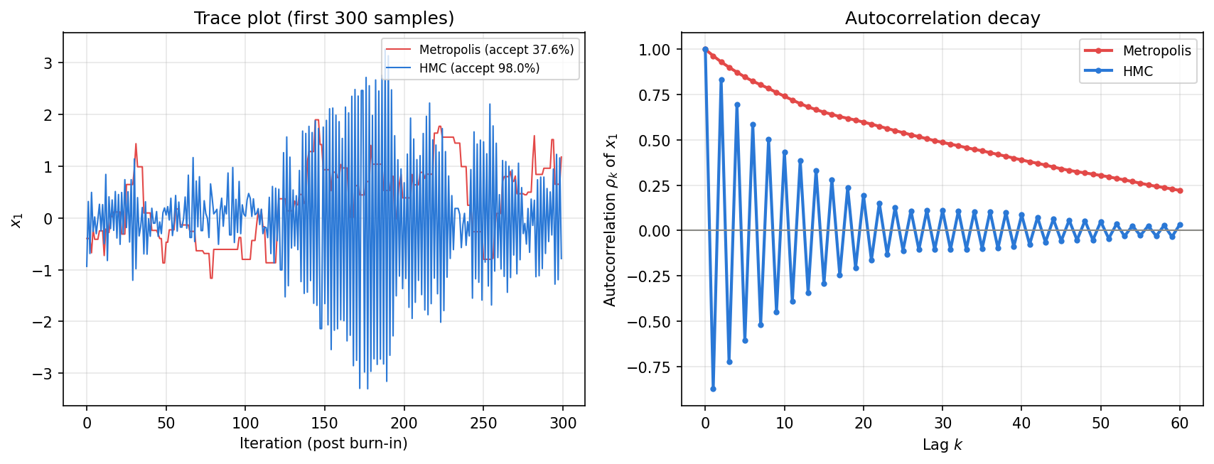
In the trace plot (left), HMC (blue) rapidly sweeps back and forth across the \(x_1\) axis, filling the whole distribution, while Metropolis (red) shows a “sticky” motion that lingers nearby. The autocorrelation function (right) makes the difference even clearer: HMC’s autocorrelation flips sign at lag 1 and oscillates while decaying rapidly to zero, whereas Metropolis shows a slow, monotonic decay that still sits around 0.2 even at lag 60. This oscillation (negative autocorrelation) is a direct consequence of a single leapfrog trajectory sweeping far across the valley in one proposal, and shows up as an integrated autocorrelation time \(\tau_{\mathrm{int}}\) of 1.000 for HMC (hitting the theoretical lower bound — essentially independent samples) versus 73.7 for Metropolis, a 73.7x gap (this individual measurement uses the same methods and sample sequences as the covariance-recovery section above but a different ESS estimator, so it won’t exactly match the 45x figure reported there — both are consistent in showing an efficiency gap of several dozen-fold).
Divergent Trajectories: When the Step Size Is Too Large
So far we’ve treated the step size \(\epsilon\) as “some appropriately chosen value.” But the first problem practitioners hit when using HMC is that when the step size is too large, leapfrog integration loses energy conservation and the simulation “diverges.” The “divergent transitions” warnings that Stan and PyMC raise refer to exactly this phenomenon (Betancourt, 2017).
Why It Diverges: A Linear Stability Analysis
For a Gaussian target \(\mathcal{N}(\mathbf{0}, \Sigma)\) , leapfrog integration decomposes along the eigenvectors of the precision matrix \(\Lambda = \Sigma^{-1}\) , and each eigenvalue’s direction behaves like a simple harmonic oscillator with angular frequency \(\omega_i = \sqrt{\lambda_i}\) . Leapfrog (a second-order explicit method) has a linear stability limit for this harmonic oscillator: beyond the following threshold, numerical error grows exponentially.
\[ \epsilon < \epsilon_{\mathrm{crit}} = \frac{2}{\sqrt{\lambda_{\max}}} \tag{5} \]where \(\lambda_{\max}\) is the largest eigenvalue of the precision matrix \(\Lambda\) . For this article’s correlated Gaussian (\(\rho=0.95\) ), the precision matrix’s eigenvalues are approximately \(0.513\) and \(20.0\) , predicting \(\epsilon_{\mathrm{crit}} = 2/\sqrt{20.0} \approx 0.447\) .
Numerical Experiment: Tracking Energy Error and Acceptance Rate as Step Size Increases
Fixing \(L=20\)
, we swept the step size from \(0.05\)
to \(1.3\)
, generating 3000 proposals at each step size and recording the mean energy error \(\overline{|\Delta H|}\)
(the average absolute difference in the Hamiltonian before/after each proposal) and the acceptance rate (seed=20260715).
def hmc_energy_error(log_prob, grad_log_prob, n_samples, step_size, n_leapfrog, x0, rng):
    x = x0.copy()
    n_accept = 0
    abs_dH = np.zeros(n_samples)
    for i in range(n_samples):
        p0 = rng.standard_normal(len(x0))
        x_new, p_new = leapfrog(x.copy(), p0.copy(), grad_log_prob, step_size, n_leapfrog)
        current_H = -log_prob(x) + 0.5 * p0 @ p0
        with np.errstate(over="ignore", invalid="ignore"):
            proposed_H = -log_prob(x_new) + 0.5 * p_new @ p_new
        if not np.isfinite(proposed_H):
            proposed_H = 1e12  # substitute a large finite value on overflow ("certain rejection")
        abs_dH[i] = abs(proposed_H - current_H)
        if np.log(rng.uniform()) < current_H - proposed_H:
            x, n_accept = x_new, n_accept + 1
    return n_accept / n_samples, abs_dH.mean()


eigvals = np.linalg.eigvalsh(Sigma_inv)
eps_crit = 2 / np.sqrt(eigvals.max())
print(f"Precision matrix eigenvalues: {eigvals}, theoretical divergence limit eps_crit={eps_crit:.3f}")

for eps in [0.05, 0.1, 0.2, 0.3, 0.4, 0.45, 0.5, 0.6, 0.7, 0.85, 1.0, 1.3]:
    rng = np.random.default_rng(20260715)
    acc, mean_dH = hmc_energy_error(log_prob, grad_log_prob, 3000, eps, 20, np.zeros(2), rng)
    print(f"eps={eps:5.2f}  accept={acc*100:6.2f}%  mean|dH|={mean_dH:.4g}")
Precision matrix eigenvalues: [ 0.51282051 20.        ], theoretical divergence limit eps_crit=0.447
eps= 0.05  accept= 99.73%  mean|dH|=0.007922
eps= 0.10  accept= 99.57%  mean|dH|=0.01297
eps= 0.20  accept= 98.17%  mean|dH|=0.03868
eps= 0.30  accept= 82.27%  mean|dH|=0.3823
eps= 0.40  accept= 83.20%  mean|dH|=0.3629
eps= 0.45  accept=  0.23%  mean|dH|=7.751e+04
eps= 0.50  accept=  0.00%  mean|dH|=3.325e+16
eps= 0.60  accept=  0.00%  mean|dH|=2.599e+27
eps= 0.70  accept=  0.00%  mean|dH|=5.279e+34
eps= 0.85  accept=  0.00%  mean|dH|=8.673e+42
eps= 1.00  accept=  0.00%  mean|dH|=2.279e+49
eps= 1.30  accept=  0.00%  mean|dH|=1.731e+59
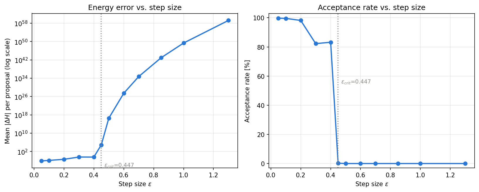
Right around the theoretical divergence threshold \(\epsilon_{\mathrm{crit}} \approx 0.447\) , the mean energy error jumps from 0.36 to 77,506 — nearly five orders of magnitude — and the acceptance rate collapses from 83.2% to 0.23%. Beyond \(\epsilon=0.5\) , the energy error exceeds \(10^{16}\) and the acceptance rate is flatly 0%. As predicted by the linear stability analysis, this happens because leapfrog integration includes a mode (the “fast” direction with eigenvalue 20) that diverges exponentially. Two practical lessons follow:
- A sharp drop in acceptance rate is a clear signal that the step size is too large. Watching the acceptance rate and adjusting the step size (e.g., dual-averaging adaptation) is a bare minimum safeguard against divergence.
- Monitoring the energy error directly catches problems earlier. Even before the acceptance rate visibly drops (\(\epsilon=0.3\) -\(0.4\) ), the energy error has already grown to roughly 40x its value at small step sizes — validating why Stan/PyMC flag individual proposals as “divergent transitions” (a more sensitive diagnostic than simply monitoring the acceptance rate).
Sensitivity to Step Size and Number of Leapfrog Steps: ESS per Gradient Evaluation as the Right Metric
The acceptance rate and ESS we’ve seen so far measure “quality per proposal,” but HMC’s computational cost scales with the number of leapfrog steps \(L\) (each proposal costs \(L+1\) gradient evaluations). So ESS per sample (the 100% reported at the top of this article, versus Metropolis’s 2.20%) alone doesn’t correctly measure computational efficiency. Increasing the number of steps tends to improve ESS, but it also increases the cost of each proposal — so the metric that actually matters for comparison is ESS per gradient evaluation.
Numerical Experiment: A Grid Search Over Step Size × Number of Leapfrog Steps
We swept all 80 combinations of step size \(\epsilon \in \{0.05, 0.10, \ldots, 0.40\}\)
(restricted to below the \(0.447\)
divergence onset) and number of leapfrog steps \(L \in \{5, 10, 20, 30, 40, 60, 80, 120, 160, 200\}\)
, generating 3000 samples each (300 burn-in, seed=20260715), computing ESS via Geyer’s initial positive sequence estimator, and normalizing by \(L+1\)
gradient evaluations.
step_sizes = [0.05, 0.10, 0.15, 0.20, 0.25, 0.30, 0.35, 0.40]
n_leapfrogs = [5, 10, 20, 30, 40, 60, 80, 120, 160, 200]
n_samples, burn = 3000, 300

results = []
for eps in step_sizes:
    for L in n_leapfrogs:
        rng = np.random.default_rng(20260715)
        samples, acc = hmc(log_prob, grad_log_prob, n_samples, eps, L, np.zeros(2), rng)
        s = samples[burn:]
        ess_x0, _ = ess_geyer(s[:, 0])
        ess_x1, _ = ess_geyer(s[:, 1])
        ess_min = min(ess_x0, ess_x1)
        grad_evals = n_samples * (L + 1)
        results.append((eps, L, acc, ess_min, ess_min / grad_evals))
A representative excerpt (of all 80 combinations; units are ESS/gradient-evaluation \(\times 10^{-3}\) ):
| \(\epsilon\) | \(L\) | Acceptance | ESS (min dim) | ESS/grad-eval (\(\times10^{-3}\) ) |
|---|---|---|---|---|
| 0.10 | 5 | 98.80% | 70.8 | 3.94 |
| 0.10 | 10 | 98.27% | 399.3 | 12.10 |
| 0.10 | 20 | 99.57% | 2034.1 | 32.29 |
| 0.10 | 80 | 98.23% | 178.4 | 0.73 |
| 0.15 | 60 | 99.33% | 22.1 | 0.12 |
| 0.25 | 10 | 91.77% | 2700.0 | 81.82 (grid maximum) |
| 0.30 | 30 | 97.83% | 21.4 | 0.23 |
| 0.35 | 200 | 71.80% | 5.2 | 0.01 |
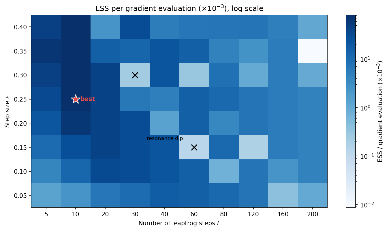
This heatmap reveals two important facts.
(1) “More leapfrog steps is always better” is false. The best point in this grid was \(\epsilon=0.25, L=10\) , with ESS/grad-eval of \(81.8\times10^{-3}\) . Around \(L=10\) , proposals are already nearly independent (ESS \(\approx\) sample count), so increasing \(L\) further barely improves per-proposal ESS while gradient-evaluation cost keeps growing linearly — so ESS/grad-eval monotonically worsens.
(2) Certain \((\epsilon, L)\) combinations are dangerous: high acceptance but collapsed ESS. For example, at \(\epsilon=0.15, L=60\) , the acceptance rate looks healthy at 99.3%, but ESS (min dimension) collapses to just 22.1 (the same \(\epsilon\) with \(L=20\) or \(L=40\) hits the 2700.0 ceiling — the sample count). This is a resonance (periodicity) phenomenon: when the trajectory length \(L\epsilon\) approaches the period of the harmonic oscillator (or an integer multiple of it), the leapfrog trajectory returns to nearly the same phase, so the proposal effectively “stays put.” Neal (2011) identifies this phenomenon theoretically, showing that a fixed \((L, \epsilon)\) combination that happens to coincide with this resonance can make the chain lose ergodicity even with a high acceptance rate, and proposes randomizing \(\epsilon\) or \(L\) on each proposal as a remedy.
This fact — that the optimal \(L\) depends on the target distribution’s shape, and that fixing it carries a hidden resonance trap — is exactly the motivation behind NUTS (the No-U-Turn Sampler), described next, which determines \(L\) automatically.
Why HMC/NUTS Is the Modern Default
This efficiency gap is exactly why modern probabilistic programming languages — Stan, PyMC, NumPyro — default to HMC (or its auto-tuning extension, NUTS: the No-U-Turn Sampler) as their sampler. When working with high-dimensional, highly-correlated posteriors in practice (e.g., hierarchical Bayesian models), basic Metropolis often can’t produce converged samples in a reasonable amount of time, making gradient-based HMC-family methods close to essential.
The Problem NUTS Solves: Manually Tuning the Number of Leapfrog Steps
As the previous section showed, the optimal number of leapfrog steps \(L\) depends on the target distribution’s shape (its eigenvalue spectrum), and fixing it risks a resonance-induced collapse in performance. Too small an \(L\) reverts to inefficient, near-random-walk exploration (at \(L=5\) , ESS/grad-eval was less than 1/20th of the optimum); too large wastes computation and can cause the trajectory to circle back near its starting point (a “U-turn”), wasting many of the gradient evaluations spent getting there.
NUTS, proposed by Hoffman & Gelman (2014), automates this manual tuning of \(L\) . Concretely, it builds a binary tree by doubling the trajectory forward and backward from the current position, and stops extending the tree the moment the dot product between momentum and position at either end of the tree turns negative (i.e., the trajectory starts curving back — a “U-turn”). This lets \(L\) be determined automatically every iteration based on the target distribution’s local geometry, freeing practitioners from having to manually search over any hyperparameter besides the step size.
More recent work addresses limitations that remain in NUTS — namely that the step size \(\epsilon\) itself is still fixed globally, and that hierarchical models with “funnel” geometries need locally varying resolution. Bou-Rabee, Carpenter & Marsden (2024)’s GIST presents a general theoretical framework for locally adapting step size and trajectory length to the current position and momentum within a Gibbs-sampling scheme, unifying NUTS and randomized HMC as special cases. Modi (2024)’s ATLAS adapts the step size at every iteration from a low-rank approximation of the local Hessian, and adapts trajectory length by monitoring the U-turn condition, substantially reducing divergent transitions on posteriors with multi-scale curvature. These represent, as of 2024, state-of-the-art answers to the exact problem we demonstrated numerically here: jointly tuning \(\epsilon\) and \(L\) is hard, and fixed values harbor dangerous combinations.
Related Articles
- Markov Chain Monte Carlo (MCMC) Fundamentals: Metropolis and Gibbs Sampling - This article follows up on the autocorrelation problem noted there, solving it with a gradient-based method.
- Bayesian Optimization: Theory and Python Implementation - Relevant to using MCMC-estimated posteriors for Bayesian optimization.
- Gaussian Process Regression (GPR) in Practice - Fully Bayesian hyperparameter inference often relies on efficient MCMC methods like HMC.
- Bayesian Linear Regression Fundamentals - A contrast with analytic (non-MCMC) Bayesian inference.
- SGD and Adam: Theory and Comparison - HMC’s use of gradients has a conceptual kinship with gradient-descent optimizers; comparing the two deepens intuition for both.
References
- Neal, R. M. (2011). MCMC using Hamiltonian dynamics. In Handbook of Markov Chain Monte Carlo. Chapman & Hall/CRC.
- Hoffman, M. D., & Gelman, A. (2014). The No-U-Turn Sampler: Adaptively setting path lengths in Hamiltonian Monte Carlo. Journal of Machine Learning Research, 15(1), 1593-1623.
- Betancourt, M. (2017). A conceptual introduction to Hamiltonian Monte Carlo. arXiv:1701.02434.
- Bou-Rabee, N., Carpenter, B., & Marsden, M. (2024). GIST: Gibbs self-tuning for locally adaptive Hamiltonian Monte Carlo. arXiv:2404.15253.
- Modi, C. (2024). ATLAS: Adapting trajectory lengths and step-size for Hamiltonian Monte Carlo. arXiv:2410.21587.