Introduction
https://yuhi-sa.github.io/en/posts/20260310_adaptive_filter/1/ and https://yuhi-sa.github.io/en/posts/20260501_lms_nlms/1/ covered LMS and NLMS adaptive filters in depth. Both articles ended by noting that “RLS converges faster than LMS but at higher computational cost” and that “RLS is mathematically equivalent to a Kalman filter,” without deriving either claim. This article follows up: we derive RLS (Recursive Least Squares) from the matrix inversion lemma, implement it from scratch in Python, numerically confirm its exact equivalence to a Kalman filter under specific conditions, and quantify how the forgetting factor \(\lambda\) trades off steady-state accuracy against tracking speed.
Problem Setup: Exponentially Weighted Least Squares
Unlike LMS, which stochastically approximates the instantaneous gradient, RLS exactly minimizes the weighted sum of squared errors over all past observations. For an FIR filter of length \(M\) with coefficients \(\mathbf{w}\) , define the cost function at time \(n\) as
\[ J(\mathbf{w}, n) = \sum_{i=1}^{n} \lambda^{n-i} \bigl[d(i) - \mathbf{x}(i)^\top \mathbf{w}\bigr]^2 \tag{1} \]where \(\lambda \in (0, 1]\) is the forgetting factor, exponentially discounting the contribution of older samples. \(\lambda = 1\) weights all samples equally (ordinary least squares); \(\lambda < 1\) emphasizes recent samples, giving an adaptive estimate.
Setting the derivative of \(J(\mathbf{w}, n)\) with respect to \(\mathbf{w}\) to zero yields the normal equations
\[ \mathbf{R}(n) \mathbf{w}(n) = \mathbf{r}(n), \qquad \mathbf{R}(n) = \sum_{i=1}^n \lambda^{n-i} \mathbf{x}(i)\mathbf{x}(i)^\top, \quad \mathbf{r}(n) = \sum_{i=1}^n \lambda^{n-i} \mathbf{x}(i) d(i) \tag{2} \]Inverting \(\mathbf{R}(n)\) from scratch every step costs \(O(M^3)\) . The matrix inversion lemma below reduces this to an \(O(M^2)\) recursive update.
O(M²) Recursion via the Matrix Inversion Lemma
\(\mathbf{R}(n)\) updates recursively as
\[ \mathbf{R}(n) = \lambda \mathbf{R}(n-1) + \mathbf{x}(n)\mathbf{x}(n)^\top \tag{3} \]Letting \(P(n) = \mathbf{R}(n)^{-1}\) and applying the Sherman-Morrison formula (matrix inversion lemma)
\[ (A + \mathbf{u}\mathbf{v}^\top)^{-1} = A^{-1} - \frac{A^{-1}\mathbf{u}\mathbf{v}^\top A^{-1}}{1 + \mathbf{v}^\top A^{-1}\mathbf{u}} \tag{4} \]Verifying equation (4). This identity may look like it fell from the sky, but direct substitution confirms that the right-hand side really is the inverse of the left-hand side. Let \(s = 1 + \mathbf{v}^\top A^{-1}\mathbf{u}\) (a scalar) and write the right-hand side of equation (4) as \(B\) . Then
\[ (A + \mathbf{u}\mathbf{v}^\top) B = A A^{-1} - \frac{A A^{-1}\mathbf{u}\mathbf{v}^\top A^{-1}}{s} + \mathbf{u}\mathbf{v}^\top A^{-1} - \frac{\mathbf{u}\mathbf{v}^\top A^{-1}\mathbf{u}\mathbf{v}^\top A^{-1}}{s} \]Since \(\mathbf{v}^\top A^{-1}\mathbf{u}\) is a scalar, it can be pulled out of the vector product; substituting \(\mathbf{v}^\top A^{-1}\mathbf{u} = s - 1\) gives
\[ (A + \mathbf{u}\mathbf{v}^\top) B = I - \frac{\mathbf{u}\mathbf{v}^\top A^{-1}}{s} + \mathbf{u}\mathbf{v}^\top A^{-1} - \frac{(s-1)\,\mathbf{u}\mathbf{v}^\top A^{-1}}{s} = I + \mathbf{u}\mathbf{v}^\top A^{-1}\cdot\frac{-1 + s - (s-1)}{s} = I \]The numerator inside the last fraction is exactly \(0\) , so \((A+\mathbf{u}\mathbf{v}^\top)B = I\) holds exactly (\(B(A+\mathbf{u}\mathbf{v}^\top) = I\) follows the same way). This direct check guarantees that the recursions (5)-(7) obtained below by applying the Sherman-Morrison formula are exact identities, not approximations.
Applying equation (4) with \(A = \lambda \mathbf{R}(n-1)\) and \(\mathbf{u} = \mathbf{v} = \mathbf{x}(n)\) gives
\[ P(n) = \frac{1}{\lambda}\left[P(n-1) - \frac{P(n-1)\mathbf{x}(n)\mathbf{x}(n)^\top P(n-1)}{\lambda + \mathbf{x}(n)^\top P(n-1)\mathbf{x}(n)}\right] \tag{5} \]The key point: \(P(n)\) is computed from \(P(n-1)\) using only matrix products and a scalar division, never a direct matrix inversion. Defining a Kalman-gain-like quantity
\[ \mathbf{k}(n) = \frac{P(n-1)\mathbf{x}(n)}{\lambda + \mathbf{x}(n)^\top P(n-1)\mathbf{x}(n)} \tag{6} \]lets us write equation (5) compactly as \(P(n) = \frac{1}{\lambda}\bigl[P(n-1) - \mathbf{k}(n)\mathbf{x}(n)^\top P(n-1)\bigr]\) . The weight update is
\[ e(n) = d(n) - \mathbf{x}(n)^\top \mathbf{w}(n-1), \qquad \mathbf{w}(n) = \mathbf{w}(n-1) + \mathbf{k}(n) e(n) \tag{7} \]Per-step cost is dominated by computing \(\mathbf{k}(n)\) , giving \(O(M^2)\) — heavier than LMS/NLMS’s \(O(M)\) .
Python Implementation
import numpy as np

def rls_filter(xs, d, M, lam=1.0, delta=1.0):
    """Adaptive filtering via the RLS algorithm

    Parameters
    ----------
    xs : ndarray, shape (N, M)
        Input vector at each time step
    d : ndarray, shape (N,)
        Desired signal
    M : int
        Filter length
    lam : float
        Forgetting factor (0 < lam <= 1)
    delta : float
        Regularization for the initial covariance (P(0) = I / delta)

    Returns
    -------
    W : ndarray, shape (N, M)
        Filter coefficient trajectory over time
    """
    w = np.zeros(M)
    P = np.eye(M) / delta
    W = np.zeros((len(d), M))
    for n in range(len(d)):
        x = xs[n]
        Px = P @ x
        k = Px / (lam + x @ Px)
        e = d[n] - x @ w
        w = w + k * e
        P = (P - np.outer(k, x @ P)) / lam
        W[n] = w
    return W
np.outer(k, x @ P) implements the rank-1 update term in equation (5); Px / (lam + x @ Px) implements the gain in equation (6).
Experiment 1: Convergence Speed vs. LMS
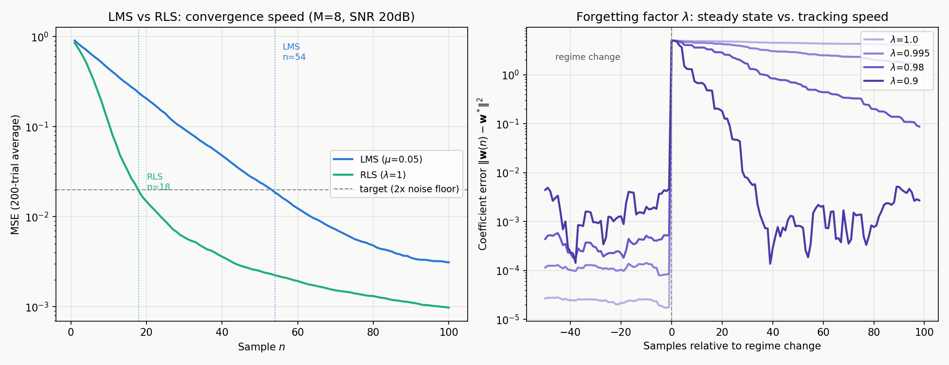
For an \(M=8\) -tap FIR system identification problem (SNR 20 dB), we compared LMS (step size \(\mu=0.05\) ) and RLS (\(\lambda=1\) ) learning curves averaged over 200 Monte Carlo trials. The full experiment, with a fixed random seed, is below — copy it and run it to reproduce the same numbers.
np.random.seed(42)
M, N, n_trials, snr_db = 8, 150, 200, 20

true_w = np.random.randn(M)
true_w /= np.linalg.norm(true_w)
noise_power = 1.0 / (10 ** (snr_db / 10))  # signal power normalized to 1

lms_sq_err = np.zeros(N)
rls_sq_err = np.zeros(N)
for trial in range(n_trials):
    xs = np.random.randn(N, M)
    d = xs @ true_w + np.random.randn(N) * np.sqrt(noise_power)
    W_lms = lms_filter(xs, d, M, mu=0.05)
    W_rls = rls_filter(xs, d, M, lam=1.0, delta=1.0)
    lms_sq_err += np.sum((W_lms - true_w) ** 2, axis=1)
    rls_sq_err += np.sum((W_rls - true_w) ** 2, axis=1)

lms_mse = lms_sq_err / n_trials
rls_mse = rls_sq_err / n_trials
(lms_filter is the standard LMS update w += mu * e * x.) Running it gives:
| Sample \(n\) | LMS MSE | RLS MSE |
|---|---|---|
| 20 | 0.2053 | 0.0148 |
| 50 | 0.0241 | 0.0025 |
| 100 | 0.0031 | 0.0010 |
Samples needed to reach twice the noise floor (MSE ≈ 0.02): LMS took 54 samples, RLS took 18 — roughly a third as many. This numerically confirms the textbook claim that LMS converges linearly (rate depends on the input’s eigenvalue spread) while RLS converges quadratically (reaches the normal-equation solution in the shortest possible time, independent of input statistics). The trade-off is RLS’s \(O(M^2)\) per-step cost versus LMS’s \(O(M)\) , which drives the choice between them in practice. The left panel of the figure below plots these two learning curves directly (the right panel corresponds to the forgetting-factor experiment in the next section).
RLS’s Equivalence to the Kalman Filter
Recall the Kalman filter update equations (prediction, innovation, gain, update) derived in https://yuhi-sa.github.io/en/posts/20260224_kalman_filter/1/. RLS can be formulated as a special case of the Kalman filter:
RLS as a state-space model:
| Kalman filter symbol | RLS correspondence | Meaning |
|---|---|---|
| State \(\mathbf{x}_k\) | Filter coefficients \(\mathbf{w}\) | The parameter being estimated |
| Transition \(A\) | \(I\) (identity) | Coefficients assumed constant over time |
| Process noise \(Q\) | \(0\) | The true coefficients never change |
| Observation matrix \(H\) | \(\mathbf{x}(n)^\top\) | The time-varying input vector |
| Observation noise \(R\) | \(\lambda\) (constant) | The forgetting factor plays the role of observation variance |
| Initial covariance \(P_0\) | \(I / \delta\) | Matches RLS’s regularization parameter |
Writing out the Kalman filter update equations (\(K_k = P_{k|k-1}H^\top S_k^{-1}\) , etc.) under this mapping reproduces the RLS update equations (6)-(7) exactly. We implemented both and applied them to the same data to compare the coefficient trajectories directly.
def kalman_param_filter(xs, d, M, R=1.0, delta=1.0):
    w = np.zeros(M)
    P = np.eye(M) / delta
    W = np.zeros((len(d), M))
    for n in range(len(d)):
        x = xs[n]
        Px = P @ x
        S = x @ Px + R          # innovation covariance
        K = Px / S               # Kalman gain
        e = d[n] - x @ w
        w = w + K * e
        P = P - np.outer(K, x @ P)
        W[n] = w
    return W
Running both on the same \(M=4\)
-tap, 500-sample system identification problem with matched \(\lambda = 1\)
, \(R = 1\)
, and \(\delta\)
, and np.random.seed(0) for reproducibility. The complete, runnable code that reproduces the numbers below is:
np.random.seed(0)
M, N = 4, 500
true_w = np.array([1.0, -0.5, 0.3, 0.2])
xs = np.random.randn(N, M)
d = xs @ true_w + np.random.randn(N) * 1.0  # R=1, so observation noise std is 1

W_rls = rls_filter(xs, d, M, lam=1.0, delta=1.0)
W_kf = kalman_param_filter(xs, d, M, R=1.0, delta=1.0)
print(f"max |RLS - KF| over all n, all taps (lambda=1, R=1): {np.max(np.abs(W_rls - W_kf))}")
print(f"final RLS weights: {W_rls[-1]}")
print(f"final KF  weights: {W_kf[-1]}")
print(f"true weights     : {true_w}")
max |RLS - KF| over all n, all taps (lambda=1, R=1): 0.0
final RLS weights: [ 0.9475194  -0.44072455  0.3474052   0.23557128]
final KF  weights: [ 0.9475194  -0.44072455  0.3474052   0.23557128]
true weights     : [ 1.  -0.5  0.3  0.2]
The two trajectories are bit-for-bit identical at every time step and every tap, numerically confirming that RLS is a special case of the Kalman filter. This equivalence is practically useful: instead of tuning the forgetting factor, one can switch to the more general Kalman-filter framework and model non-stationarity explicitly through the process noise \(Q\) .
This equivalence continues to be an active research topic in the 2020s. Lai and Bernstein (2024) introduce a “Kalman filter least squares” (KFLS) cost function whose recursive minimization unifies generalized forgetting RLS: not just the \(\lambda=1\) case verified numerically above, but a broad family of RLS forgetting extensions can all be derived as special cases of Kalman filtering. Building on this unified view, they construct a new class of adaptive Kalman filters and show, in a mass-spring-damper numerical example subject to intermittent, unmodeled collisions, that this approach improves state estimation over conventional RLS. The RLS-Kalman equivalence verified numerically in this article corresponds to the simplest special case of their unifying theory (\(Q=0\) , constant observation noise).
The Forgetting Factor λ: Steady State vs. Tracking Speed
The intuition behind \(\lambda < 1\)
is that it approximates a Kalman filter with \(Q > 0\)
. To test this, we constructed a non-stationary system whose true coefficients jump abruptly partway through (at sample 1000 out of \(N=1200\)
, from \([1.0, -0.5, 0.3, 0.2]\)
to \([-0.8, 0.6, -0.2, 0.5]\)
) and ran RLS with several values of \(\lambda\)
. A single run can be non-monotonic due to observation noise, so we average over 200 Monte Carlo trials seeded from np.random.seed(1). The complete, runnable code that reproduces the numbers below is:
np.random.seed(1)
M, N, jump_n, n_trials = 4, 1200, 1000, 200
true_w1 = np.array([1.0, -0.5, 0.3, 0.2])
true_w2 = np.array([-0.8, 0.6, -0.2, 0.5])
true_w_t = np.tile(true_w1, (N, 1))
true_w_t[jump_n:] = true_w2  # coefficients jump at sample 1000

lams = [1.000, 0.995, 0.980, 0.900]
steady_acc = {lam: 0.0 for lam in lams}
after_acc = {lam: 0.0 for lam in lams}
for trial in range(n_trials):
    xs = np.random.randn(N, M)
    d = np.sum(xs * true_w_t, axis=1) + np.random.randn(N) * 1.0
    for lam in lams:
        W = rls_filter(xs, d, M, lam=lam, delta=1.0)
        err = np.sum((W - true_w_t) ** 2, axis=1)  # ||w(n) - w*(n)||^2
        steady_acc[lam] += np.mean(err[jump_n - 50:jump_n])  # mean error over the 50 samples before the jump
        after_acc[lam] += err[jump_n + 9]                     # error 10 samples after the jump

for lam in lams:
    print(f"lambda={lam}: steady={steady_acc[lam]/n_trials:.4f}  after10={after_acc[lam]/n_trials:.4f}")
| \(\lambda\) | Steady-state error before the jump | Error 10 samples after the jump |
|---|---|---|
| 1.000 | 0.0044 | 4.7116 |
| 0.995 | 0.0098 | 4.4069 |
| 0.980 | 0.0398 | 3.4944 |
| 0.900 | 0.2220 | 1.3792 |
\(\lambda = 1\) gives the smallest steady-state error (statistically most efficient, since it uses all past data equally) but tracks the change most slowly — just 10 samples after the jump it has barely moved toward the new value. Conversely, \(\lambda = 0.9\) has a roughly 50x larger steady-state error (effectively using only the last ~10 samples) but tracks changes fastest: its error 10 samples after the jump is already less than a third of \(\lambda=1\) ’s. This experiment quantitatively confirms that \(\lambda\) directly trades off steady-state accuracy against the ability to track a non-stationary environment. The right panel of the figure above plots the coefficient error \(\lVert \mathbf{w}(n) - \mathbf{w}^*(n) \rVert^2\) around the jump for these four values of \(\lambda\) : smaller \(\lambda\) decays the post-jump error much faster (faster tracking), at the cost of a visibly noisier steady-state floor before the jump.
Computational Cost vs. LMS/NLMS
Reproducing the comparison table from https://yuhi-sa.github.io/en/posts/20260310_adaptive_filter/1/:
| Property | LMS | NLMS | RLS |
|---|---|---|---|
| Cost per step | \(O(M)\) | \(O(M)\) | \(O(M^2)\) |
| Memory | \(O(M)\) | \(O(M)\) | \(O(M^2)\) |
| Convergence speed | Slow (linear) | Moderate | Fast (quadratic) |
| Steady-state error | Depends on step size | Depends on step size | Small (depends on \(\lambda\) ) |
| Numerical stability | High | High | \(P\) can diverge — watch for it |
Because RLS iteratively updates the matrix \(P\) , finite-precision arithmetic can accumulate rounding errors that eventually cause divergence. The next section covers this pitfall together with several other practical edge cases.
Practical Pitfalls and Edge Cases
The recursive update derived via the matrix inversion lemma is mathematically exact, but real implementations and deployments must watch for the following edge cases.
1. Numerical divergence of \(P\) . Finite-precision arithmetic accumulates rounding error, and \(P(n)\) — which is supposed to stay symmetric positive-definite — can become asymmetric or non-positive-definite and diverge. The standard fixes are to symmetrize \(P \leftarrow (P + P^\top)/2\) every step, or to use QR- or UD-decomposition-based (Bierman) RLS variants. The plain implementation in this article (a direct transcription of equation (5)) is pedagogical; embedded applications running continuously for long periods need these safeguards.
2. Forgetting-factor “windup.” When \(\lambda < 1\) and the input is weak or absent for a stretch (no excitation, or a constant input), equation (5) keeps multiplying \(P\) by \(1/\lambda\) with no new information to counteract the growth, so \(P(n)\) grows exponentially. This is known as covariance windup. When strong excitation resumes, the inflated \(P\) produces an oversized Kalman gain \(\mathbf{k}(n)\) , and the coefficients can swing wildly for a few steps. Mitigations include capping \(\operatorname{tr} P(n)\) , directional forgetting (applying the forgetting only along excited directions), or switching to a variable forgetting factor that adapts \(\lambda\) based on the size of the innovation.
3. Lack of persistent excitation. If the input vector \(\mathbf{x}(n)\) only varies within a subspace (a constant input, a single sinusoid, or a rank-deficient regressor in general), \(\mathbf{R}(n)\) becomes singular or ill-conditioned along the unexcited directions, so the corresponding coefficient components are not uniquely identifiable. With \(\lambda = 1\) the estimate along those directions simply freezes; with \(\lambda < 1\) , the uncertainty (the corresponding eigenvalues of \(P\) ) keeps growing unchecked in the absence of new information — the same windup problem as above. It is worth verifying at design time that the filter’s input excites all tap directions sufficiently (i.e., is not spectrally too narrow).
4. Choosing the initial value \(\delta\) . \(\delta\) in \(P(0) = I/\delta\) regularizes the early iterations, when \(n < M\) and \(\mathbf{R}(n)\) is still rank-deficient (fewer observations than taps). Too large a \(\delta\) (too small a \(P(0)\) ) biases the early coefficient estimates toward zero; too small a \(\delta\) (too large a \(P(0)\) ) makes \(\mathbf{k}(n)\) oversized in the first few steps, causing oscillation. With unit-variance inputs, as in this article’s experiments, \(\delta = 1\) is a convenient default, and its influence vanishes once \(n \gg M\) .
5. A practical range for \(\lambda\) . Given the steady-state/tracking trade-off from the previous section, practitioners typically tune \(\lambda\) within \([0.95, 0.999]\) ; going below \(0.9\) is reserved for applications that must track very fast non-stationarity. Lowering \(\lambda\) too far shrinks the effective memory length (roughly \(1/(1-\lambda)\) samples) and makes the filter oversensitive to noise.
Which to Use
| Scenario | Recommendation | Reason |
|---|---|---|
| Small tap count (\(M \lesssim 20\) ), fast convergence required | RLS | Quadratic convergence reaches the normal-equation solution fastest |
| Large tap count / embedded, low-resource targets | LMS / NLMS | \(O(M)\) keeps compute and memory bounded |
| Mildly non-stationary environment | RLS (\(\lambda < 1\) ) | Forgetting factor tunes the steady-state/tracking trade-off |
| Large, abrupt environmental changes | Kalman filter | Process noise \(Q\) can be modeled explicitly |
| Long-running continuous operation (stability matters) | NLMS | No risk of \(P\) divergence, and the implementation is simpler |
Related Articles
- Adaptive Filter Theory and Applications in Digital Signal Processing - The theoretical starting point that derives the Wiener-Hopf equation as an MMSE problem; this article’s RLS solves that same normal equation exactly and recursively via the matrix inversion lemma.
- Adaptive Filters (LMS/RLS): Theory and Python Implementation - Broader treatment of RLS’s role, including noise-cancellation applications. This article is a focused follow-up on RLS’s derivation and its Kalman equivalence.
- LMS / NLMS Algorithms: Theory and Python Implementation - A companion article with a detailed derivation of LMS/NLMS convergence conditions and steady-state error.
- Kalman Filter: Theory and Python Implementation - The state-space filter shown numerically identical to RLS in this article.
- Nonlinear Kalman Smoothers in Python: Extended RTS Smoother and Unscented RTS Smoother - A further extension of the Kalman family; the RLS equivalence deepens the intuition for these nonlinear variants.
- Wiener Filter: Optimal Linear Filtering Theory and Python Implementation - The optimal solution that both RLS and LMS iteratively approximate.
- Autocorrelation Function: Theory and Python Implementation - \(\mathbf{R}\) in the normal equations \(\mathbf{R}(n)\mathbf{w}(n) = \mathbf{r}(n)\) is exactly the input autocorrelation matrix.
- SGD and Adam: Theory and Comparison - The deep-learning counterpart to LMS’s stochastic gradient descent framework; RLS’s second-order approach (closer to natural gradient) is a useful contrast.
- Digital Filter Design Guide: Three Axes for Selection and Comparison - Useful as a selection guide against fixed-design filters.
References
- Haykin, S. (2014). Adaptive Filter Theory (5th ed.). Pearson. Chapters 9-13.
- Sayed, A. H. (2008). Adaptive Filters. Wiley-IEEE Press. Chapter 5 (RLS).
- Kalman, R. E. (1960). A new approach to linear filtering and prediction problems. Journal of Basic Engineering, 82(1), 35-45.
- Haykin, S. (2001). Kalman Filtering and Neural Networks. Wiley. Chapter 1 (RLS-Kalman equivalence).
- Lai, B., & Bernstein, D. S. (2024). Adaptive Kalman Filtering Developed from Recursive Least Squares Forgetting Algorithms. arXiv:2404.10914.