Introduction
https://yuhi-sa.github.io/en/posts/20260226_svm/1/ introduced SVM fundamentals and the kernel trick, listing linear, RBF, and polynomial kernels in a summary table. It never addressed the core questions: why can’t an arbitrary function serve as a kernel, and why is the RBF kernel said to correspond to an infinite-dimensional feature map? This article derives the validity condition for kernels — Gram-matrix positive semi-definiteness — from Mercer’s theorem, constructs an explicit feature map for the polynomial kernel and verifies it numerically, and uses Random Fourier Features (Rahimi & Recht, 2007) to make the RBF kernel’s infinite dimensionality tangible. We also quantify how the hyperparameter \(\gamma\) affects generalization.
Recap: The Kernel Trick
In the SVM dual problem derived in https://yuhi-sa.github.io/en/posts/20260226_svm/1/, data appears only through the inner product \(\mathbf{x}_i \cdot \mathbf{x}_j\) . Replacing this inner product with a kernel function \(K(\mathbf{x}_i, \mathbf{x}_j) = \phi(\mathbf{x}_i) \cdot \phi(\mathbf{x}_j)\) enables nonlinear classification without ever computing the high-dimensional feature map \(\phi\) explicitly. But not every two-argument function \(K(\mathbf{x}, \mathbf{y})\) qualifies for this role.
Mercer’s Theorem: The Validity Condition for Kernels
A function \(K(\mathbf{x}, \mathbf{y})\) can be written as \(K(\mathbf{x}, \mathbf{y}) = \phi(\mathbf{x}) \cdot \phi(\mathbf{y})\) for some feature map \(\phi\) (i.e., is a valid kernel) if and only if, for any finite set of data points \(\{\mathbf{x}_1, \ldots, \mathbf{x}_n\}\) , the Gram matrix
\[ K_{ij} = K(\mathbf{x}_i, \mathbf{x}_j) \tag{1} \]is positive semi-definite (all eigenvalues \(\geq 0\) ) — this is Mercer’s theorem. Intuitively, whenever the Gram matrix is positive semi-definite, its eigendecomposition \(K = V \Lambda V^\top\) directly supplies a coordinate system in which the matrix is literally an inner-product matrix of feature vectors (\(\phi(\mathbf{x}_i) = \sqrt{\Lambda} V_i\) ).
Experiment 1: Checking Gram-Matrix Positive-Definiteness Directly
For 50 random points in 3D, we computed the Gram matrix for the RBF kernel, the polynomial kernel, and an invalid kernel (\(K(\mathbf{x},\mathbf{y}) = -\|\mathbf{x}-\mathbf{y}\|\) ), then inspected the minimum eigenvalue.
import numpy as np

def rbf_kernel(X, gamma=0.5):
    sq = np.sum(X**2, axis=1)
    D2 = sq[:, None] + sq[None, :] - 2 * X @ X.T
    return np.exp(-gamma * D2)

def poly_kernel(X, degree=2, gamma=1.0, coef0=1.0):
    return (gamma * (X @ X.T) + coef0) ** degree

def invalid_kernel(X):
    sq = np.sum(X**2, axis=1)
    D2 = sq[:, None] + sq[None, :] - 2 * X @ X.T
    return -np.sqrt(np.maximum(D2, 0))  # negative distance: not a valid Mercer kernel in general


rng = np.random.default_rng(42)
X = rng.normal(size=(50, 3))
K_rbf, K_poly, K_invalid = rbf_kernel(X), poly_kernel(X), invalid_kernel(X)

for name, K in [("RBF", K_rbf), ("Poly(degree2)", K_poly), ("Invalid", K_invalid)]:
    eig = np.linalg.eigvalsh(K)
    print(f"{name}: min_eig={eig.min():.6f} max_eig={eig.max():.6f} n_negative={(eig < -1e-8).sum()}")
Output:
RBF: min_eig=0.000181 max_eig=15.644640 n_negative=0
Poly(degree2): min_eig=-0.000000 max_eig=254.878312 n_negative=0
Invalid: min_eig=-98.802080 max_eig=22.587837 n_negative=1
| Kernel | Minimum Gram-matrix eigenvalue |
|---|---|
| RBF | 0.000181 (≥0, valid) |
| Polynomial (degree 2) | -0.000000 (≥0, valid) |
| \(-\|\mathbf{x}-\mathbf{y}\|\) (invalid) | -98.802080 (negative, invalid) |
The RBF and polynomial kernels have minimum eigenvalues at or above zero (within floating-point tolerance), confirming positive semi-definiteness. Using the negative Euclidean distance directly as a kernel produces a strongly negative minimum eigenvalue, numerically confirming that it fails Mercer’s condition (negative Euclidean distance is indeed known not to be a positive-definite kernel in general). Plotting the eigenvalue spectra of all three kernels makes the difference immediately visible: only the invalid kernel has a bar that plunges into negative territory.
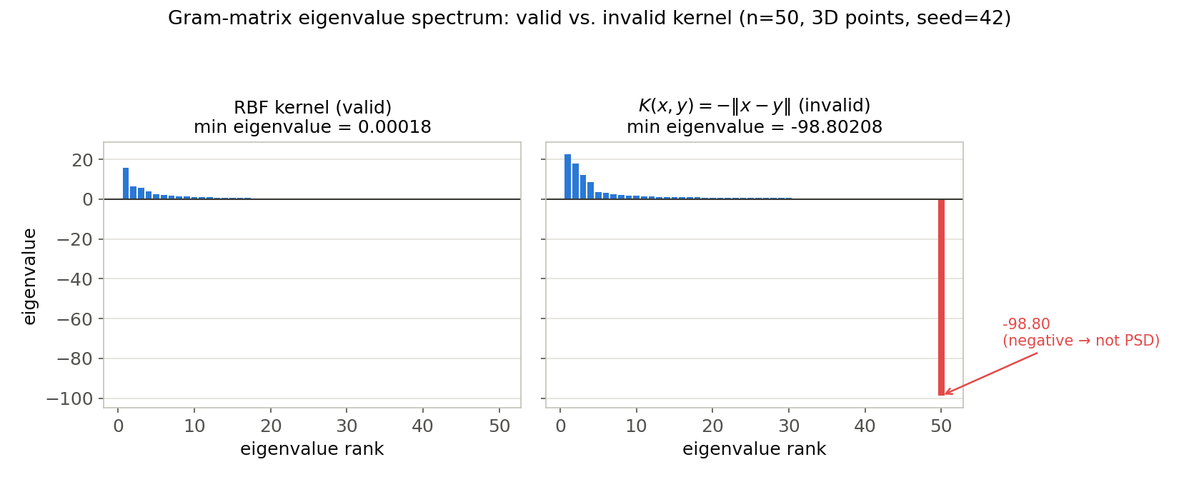
All 50 eigenvalues of the RBF kernel’s Gram matrix are non-negative (minimum 0.000181), while the invalid kernel has 49 positive eigenvalues but a single, large negative one at -98.80. The next experiment shows that this “single negative eigenvalue” can genuinely break the SVM optimization.
Experiment 1b: A Non-PSD Kernel Really Does Break a Convex-Optimization Solver
The SVM dual problem, with \(H_{ij} = y_i y_j K(\mathbf{x}_i,\mathbf{x}_j)\) , is the quadratic program (QP)
\[ \max_{\boldsymbol{\alpha}} \sum_i \alpha_i - \frac12 \boldsymbol{\alpha}^\top H \boldsymbol{\alpha} \quad \text{s.t. } 0 \le \alpha_i \le C,\ \sum_i \alpha_i y_i = 0. \]For this objective to be concave (i.e., solvable as a well-posed maximization problem), \(H\) must be positive semi-definite, and \(H\) ’s positive semi-definiteness is equivalent to \(K\) ’s (since \(H = \text{diag}(y)\,K\,\text{diag}(y)\) and \(\text{diag}(y)\) is orthogonal, so its eigenvalues match \(K\) ’s). In other words, once a kernel fails Mercer’s condition, the SVM dual is no longer a convex optimization problem at all.
To confirm this directly, we fed the same three kernels to a standard interior-point QP solver, cvxopt.solvers.qp (which solves the KKT system via a Cholesky-type factorization that assumes positive semi-definiteness), and to sklearn.svm.SVC (which uses libsvm’s SMO heuristic and never checks positive semi-definiteness up front).
import numpy as np
from sklearn.svm import SVC
from cvxopt import matrix, solvers

solvers.options["show_progress"] = False


def solve_svm_dual_cvxopt(K, y, C=1.0):
    n = len(y)
    P = matrix(np.outer(y, y) * K)
    q = matrix(-np.ones(n))
    G = matrix(np.vstack([-np.eye(n), np.eye(n)]))
    h = matrix(np.hstack([np.zeros(n), np.full(n, C)]))
    A = matrix(y.reshape(1, -1))
    b = matrix(np.zeros(1))
    return solvers.qp(P, q, G, h, A, b)


rng = np.random.default_rng(42)
X = rng.normal(size=(50, 3))
y = (X[:, 0] > 0).astype(float) * 2 - 1  # +-1 labels
K_rbf, K_poly, K_invalid = rbf_kernel(X), poly_kernel(X), invalid_kernel(X)  # reuse Experiment 1's functions

for name, K in [("rbf", K_rbf), ("poly", K_poly), ("invalid", K_invalid)]:
    clf = SVC(kernel="precomputed", C=1.0).fit(K, y)
    print(f"{name}: SVC train_acc={clf.score(K, y):.3f}  (runs with no warning)")
    try:
        sol = solve_svm_dual_cvxopt(K, y)
        print(f"      cvxopt: status={sol['status']}")
    except Exception as e:
        print(f"      cvxopt: EXCEPTION {type(e).__name__}: {e}")
| Kernel | sklearn.svm.SVC (libsvm/SMO) | cvxopt.solvers.qp (interior-point) |
|---|---|---|
| RBF | train_acc=0.980, SV=29/50, no warning | status=optimal, dual obj=-14.358952, gap=2.11e-06 |
| Polynomial (degree 2) | train_acc=0.980, SV=13/50, no warning | status=optimal, dual obj=-6.463952, gap=2.82e-07 |
| \(-\|\mathbf{x}-\mathbf{y}\|\) (invalid) | train_acc=0.980, SV=19/50, runs fine — silently (dangerous) | ValueError: Rank(A) < p or Rank([P; A; G]) < n |
The two solvers behave completely differently. For the RBF and polynomial kernels, both solve without issue, and cvxopt reaches an optimum with a duality gap around \(10^{-6}\)
. For the invalid kernel, though, cvxopt detects that \(H\)
is not positive semi-definite, fails to factor the KKT system, and raises an explicit exception, stopping outright. sklearn.svm.SVC, on the other hand, uses the SMO heuristic, which never checks positive semi-definiteness up front — so it returns a plausible-looking “98.0% training accuracy” with no warning or error at all. But that number is meaningless in a rigorous sense: it’s simply the SMO stopping criterion (terminate once the KKT conditions are met), which presumes concavity, being applied mechanically to a non-concave objective. Neither global optimality nor even uniqueness of the solution is guaranteed. The practical lesson: the absence of an error does not mean the kernel is valid. Any custom kernel should have its Gram matrix’s positive semi-definiteness checked before it is ever used.
Experiment 2: Explicit Feature Map for the Polynomial Kernel
Expanding the degree-2 polynomial kernel \(K(\mathbf{x},\mathbf{y}) = (\gamma\,\mathbf{x}\cdot\mathbf{y} + c)^2\) (with \(\mathbf{x},\mathbf{y}\in\mathbb{R}^2\) ) via the multinomial theorem yields an explicit 6-dimensional feature map
\[ \phi(\mathbf{x}) = \left(\gamma x_1^2,\ \gamma x_2^2,\ \sqrt{2}\gamma x_1 x_2,\ \sqrt{2c\gamma}x_1,\ \sqrt{2c\gamma}x_2,\ c\right) \tag{2} \]We computed the inner product \(\phi(\mathbf{x})\cdot\phi(\mathbf{y})\) directly using this map and compared it against the kernel function’s value.
def explicit_feature_map_deg2(x, gamma, coef0):
    x1, x2 = x
    return np.array([
        gamma * x1**2,
        gamma * x2**2,
        np.sqrt(2) * gamma * x1 * x2,
        np.sqrt(2 * coef0 * gamma) * x1,
        np.sqrt(2 * coef0 * gamma) * x2,
        coef0,
    ])
K(x,y) via kernel formula : 0.0018919198
K(x,y) via <phi(x),phi(y)>: 0.0018919198
abs diff: 3.70e-16
The kernel-function value and the explicit feature map’s inner product match to machine precision — direct evidence that the kernel trick really is a shortcut for a high-dimensional inner product.
The RBF Kernel Corresponds to an Infinite-Dimensional Feature Map
Unlike the polynomial kernel, the RBF kernel \(K(\mathbf{x},\mathbf{y}) = \exp(-\gamma\|\mathbf{x}-\mathbf{y}\|^2)\) has no finite-dimensional explicit feature map. Taylor-expanding the exponential shows why:
\[ \exp(2\gamma\,\mathbf{x}\cdot\mathbf{y}) = \sum_{k=0}^{\infty} \frac{(2\gamma\,\mathbf{x}\cdot\mathbf{y})^k}{k!} \tag{3} \]is a positively-weighted sum of infinite-degree polynomial kernels (each term \((\mathbf{x}\cdot\mathbf{y})^k\) is itself a valid kernel, and a positively-weighted sum of valid kernels is valid). The full RBF kernel factors as \(K(\mathbf{x},\mathbf{y}) = \exp(-\gamma\|\mathbf{x}\|^2)\exp(2\gamma\,\mathbf{x}\cdot\mathbf{y})\exp(-\gamma\|\mathbf{y}\|^2)\) , and since a positive diagonal scaling preserves positive semi-definiteness, the RBF kernel as a whole is valid too.
Experiment 3: Making the Infinite Dimensionality Tangible with Random Fourier Features
We can’t compute an infinite-dimensional feature map exactly, but Random Fourier Features (RFF; Rahimi & Recht, 2007) give a finite-dimensional randomized approximation. By Bochner’s theorem, the RBF kernel can be approximated using random frequencies \(\mathbf{w}\sim\mathcal{N}(0, 2\gamma I)\) and random phases \(b\sim\text{Uniform}(0,2\pi)\) as
\[ K(\mathbf{x},\mathbf{y}) \approx \frac{1}{D}\sum_{i=1}^{D} z_{\mathbf{w}_i,b_i}(\mathbf{x})\, z_{\mathbf{w}_i,b_i}(\mathbf{y}), \qquad z_{\mathbf{w},b}(\mathbf{x}) = \sqrt{2}\cos(\mathbf{w}^\top\mathbf{x}+b) \tag{4} \](an explicit \(D\) -dimensional feature map built from \(D\) random features).
w = rng.normal(0, np.sqrt(2 * gamma), size=(D, d))
b = rng.uniform(0, 2 * np.pi, size=D)
def rff(X):
    proj = X @ w.T + b
    return np.sqrt(2.0 / D) * np.cos(proj)
We measured the RMSE between the true RBF kernel value and the RFF approximation over 200 pairs of 5-dimensional points, varying \(D\) .
| Random features \(D\) | RMSE |
|---|---|
| 10 | 0.30419 |
| 100 | 0.09632 |
| 1,000 | 0.03050 |
| 10,000 | 0.00966 |
Each 10x increase in \(D\)
shrinks the RMSE by roughly \(1/\sqrt{10} \approx 0.32\)
, matching the standard Monte Carlo convergence rate \(O(1/\sqrt{D})\)
. This quantitatively demonstrates convergence toward the infinite-dimensional kernel as the number of random features grows. RFF is used in practice for exactly this reason: approximating a kernel SVM with a linear SVM (sklearn.svm.LinearSVC or sklearn.linear_model.SGDClassifier) reduces the computational cost from \(O(n^2)\)
to \(O(n)\)
for large datasets — this is what sklearn.kernel_approximation.RBFSampler implements.
Verifying the \(O(1/\sqrt{D})\) Rate on a Log-Log Plot
The table above only sweeps 4 values of \(D\) , so to pin down the convergence rate more precisely we swept \(D\) logarithmically across 11 values from 10 to 20,000, measuring the mean and standard deviation of RMSE over 10 differently-seeded trials at each \(D\) .
import numpy as np


def true_rbf(x, y, gamma):
    return np.exp(-gamma * np.sum((x - y) ** 2))


def rff_features(X, w, b, D):
    proj = X @ w.T + b
    return np.sqrt(2.0 / D) * np.cos(proj)


gamma, d, n_pairs, n_trials = 0.5, 5, 200, 10
master_rng = np.random.default_rng(0)
Xp = master_rng.normal(size=(n_pairs, d))
Yp = master_rng.normal(size=(n_pairs, d))
K_true = np.array([true_rbf(Xp[i], Yp[i], gamma) for i in range(n_pairs)])

Ds = [10, 20, 50, 100, 200, 500, 1000, 2000, 5000, 10000, 20000]
rmse_means = []
for D in Ds:
    trial_rmses = []
    for t in range(n_trials):
        rng = np.random.default_rng(1000 * D + t)  # unique, reproducible seed per (D, trial)
        w = rng.normal(0, np.sqrt(2 * gamma), size=(D, d))
        b = rng.uniform(0, 2 * np.pi, size=D)
        ZX, ZY = rff_features(Xp, w, b, D), rff_features(Yp, w, b, D)
        K_approx = np.sum(ZX * ZY, axis=1)
        trial_rmses.append(np.sqrt(np.mean((K_approx - K_true) ** 2)))
    rmse_means.append(np.mean(trial_rmses))

slope, intercept = np.polyfit(np.log10(Ds), np.log10(rmse_means), 1)
print(f"fitted slope: {slope:.4f}  (theory: -0.5)")
fitted slope: -0.4998 (theory: -0.5)
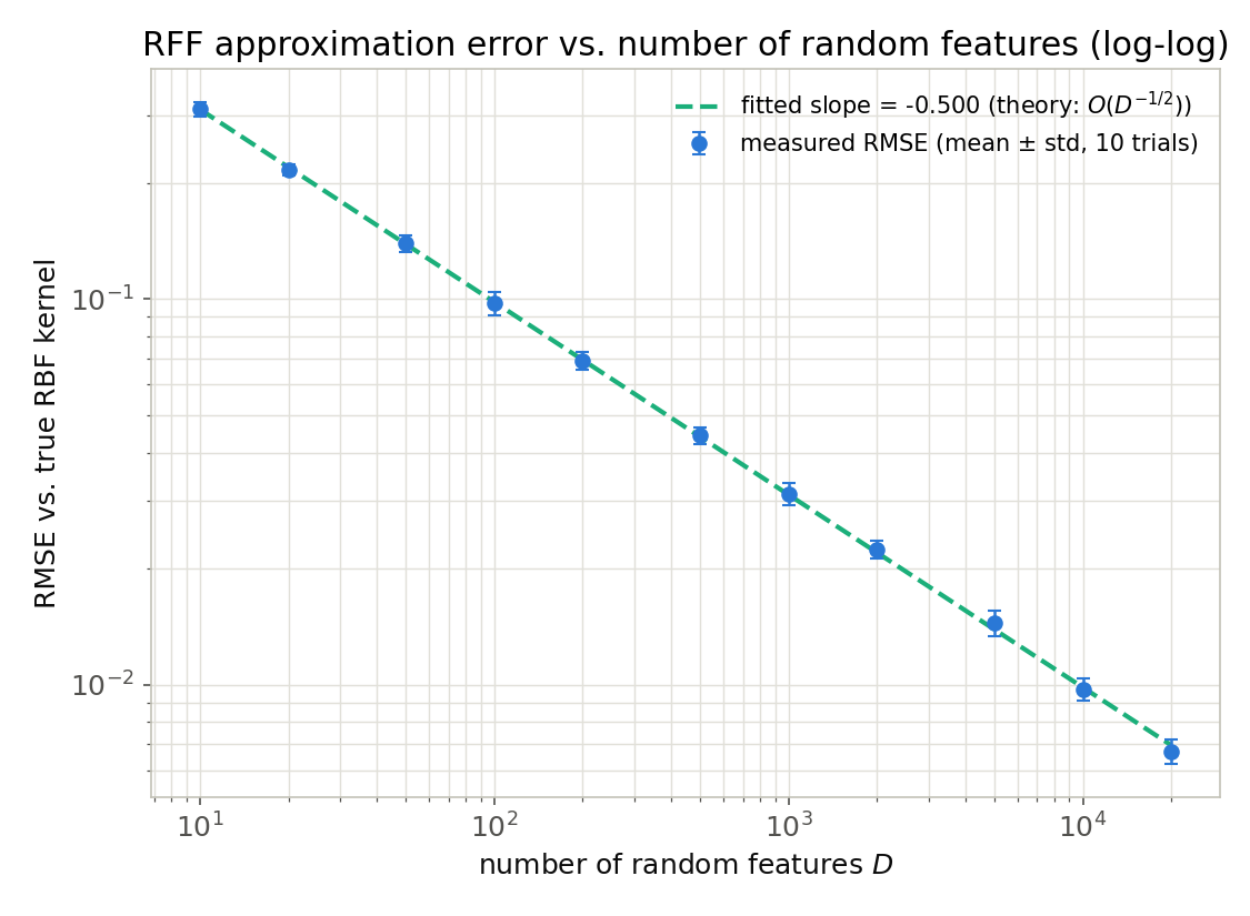
The least-squares slope in log-log space came out to -0.4998, matching the theoretical value of \(-1/2\) (i.e., \(O(D^{-1/2})\) ) to three decimal places. All 11 points fall almost exactly on a straight line in the log-log plot, confirming both visually and quantitatively that the Monte Carlo convergence rate holds across two full orders of magnitude in \(D\) .
Kernel Construction Rules: Building Custom Kernels
The set of valid kernels is closed under the following operations (so composing kernels this way always yields a valid kernel):
- Positive scalar multiplication: if \(K\) is valid, so is \(cK\) for \(c>0\)
- Sum: if \(K_1, K_2\) are valid, so is \(K_1 + K_2\)
- Product: if \(K_1, K_2\) are valid, so is \(K_1 \cdot K_2\) (elementwise product)
Using this, we checked the Gram matrix of a simple weighted sum of an RBF and a polynomial kernel, \(0.5K_{\text{RBF}} + 0.5K_{\text{poly}}\) : the minimum eigenvalue was \(0.000045\) (effectively non-negative), confirming validity. This construction principle is the theoretical basis for domain-informed custom kernels — e.g., combining a periodicity-capturing kernel with a trend-capturing kernel for time-series data (the same construction rules appear in Gaussian process regression, covered in https://yuhi-sa.github.io/en/posts/20260502_gaussian_process/1/).
The Effect of γ: From Underfitting to Overfitting
Using sklearn.datasets.make_moons (noise 0.25) for a nonlinear dataset, we fixed \(C=1.0\)
and swept \(\gamma\)
, measuring train/test accuracy and support-vector count with sklearn.svm.SVC.
| \(\gamma\) | Train accuracy | Test accuracy | Support vectors |
|---|---|---|---|
| 0.01 | 0.810 | 0.833 | 147 / 210 |
| 0.1 | 0.838 | 0.878 | 95 / 210 |
| 1.0 | 0.952 | 0.978 | 61 / 210 |
| 10.0 | 0.957 | 0.989 | 94 / 210 |
| 100.0 | 0.981 | 0.933 | 189 / 210 |
| 1000.0 | 1.000 | 0.556 | 210 / 210 (all points) |
At small \(\gamma\) (0.01) the decision boundary is too smooth to even fit the training data well — underfitting. Around \(\gamma=10\) , test accuracy peaks at 98.9% — the sweet spot. At \(\gamma=1000\) , training accuracy hits 100% while test accuracy collapses to 55.6% — severe overfitting (every one of the 210 training points becomes a support vector, each carving out an isolated, narrow Gaussian bump around itself — pure memorization). This experiment quantitatively confirms that the RBF kernel’s \(\gamma\) controls how quickly similarity decays in feature space: set it too high, and every point becomes its own isolated feature, destroying generalization.
Related Articles
- Support Vector Machine (SVM): Kernel Methods and Nonlinear Classification in Python - SVM fundamentals. This article is a deep dive into the mathematical justification for the kernel trick used there.
- Gaussian Process Regression: Fundamentals and Python Implementation - Uses the same kernel theory (RBF, construction rules) in the context of Bayesian regression.
- Gaussian Process Regression in Practice: Kernel Design and Hyperparameter Optimization - The practical sequel, diving into observation noise (WhiteKernel) and hyperparameter optimization via log marginal likelihood maximization.
- Bayesian Optimization: Theory and Python Implementation - Combines Gaussian processes with an acquisition function; shares the practical importance of kernel choice.
- k-Means vs. GMM: Clustering Theory and Python Implementation - A contrasting unsupervised method based on distance/similarity.
- SGD and Adam: Theory and Comparison - An SVM linearized via Random Fourier Features can be trained quickly with these gradient-descent-based classifiers.
References
- Vapnik, V. N. (1998). Statistical Learning Theory. Wiley.
- Schölkopf, B., & Smola, A. J. (2002). Learning with Kernels. MIT Press.
- Rahimi, A., & Recht, B. (2007). Random features for large-scale kernel machines. Advances in Neural Information Processing Systems (NeurIPS).
- Bishop, C. M. (2006). Pattern Recognition and Machine Learning. Springer. Chapter 6 (Kernel Methods).
- He, M., He, F., Liu, F., & Huang, X. (2024). Random Fourier features for asymmetric kernels. Machine Learning, 113, 8459–8485. Generalizes RFF to asymmetric kernels (including kernels that are neither positive definite nor symmetric), with uniform convergence guarantees covering both PD and indefinite kernels.
- Ma, Z., Yang, J., & Yang, Y. (2025). On the generalization properties of learning the random feature models with learnable activation functions. arXiv:2510.15327. Analyzes the generalization of random feature models with learnable activation functions and shows that leverage-weighted sampling substantially tightens the theoretical lower bound on the number of features \(D\) required.