1. Connection Pool Sizing as a Real Operational Problem
Between an application server and a database there is usually a “connection pool.” Establishing a TCP connection and authenticating with the DB is never cheap, so instead of reconnecting on every request, the application keeps a fixed number of connections open in advance and reuses them. How to size that pool, c, is a deceptively small setting that causes real operational friction.
ctoo small: The number of requests that can be handled concurrently is capped by the pool size. Once no free connection is available, requests queue up, and wait time degrades exponentially as load increases.ctoo large: Too many connections on the DB server itself can increase overhead from context switching and lock contention (multiple backend processes/threads fighting over the same rows or index pages), which can actually reduce throughput. Anyone who’s operated PostgreSQL or MySQL has probably heard the folklore that “cranking upmax_connectionscan make things slower.”
So the optimal c is a problem with a sweet spot somewhere in the middle — too small or too large both hurt — which is exactly the kind of question that’s better answered with a mathematical model and simulation than with intuition. This article formalizes the problem as an M/M/c queueing model and runs a real Python simulation to quantify both the wait-time blowup and (under a specific, honest model) the throughput peak phenomenon.
This article is a natural extension of https://yuhi-sa.github.io/en/posts/20211121_db/1/, which covers SQL basics. Where that article measured how fast a single query runs, this one asks a layer up: how many queries can you afford to run concurrently, and how should the pool be designed for that?
2. The M/M/c Queueing Model and Little’s Law
Queueing theory models a system with three parameters:
- Arrival rate \(\lambda\) : the average number of requests arriving per unit time (assuming a Poisson process — inter-arrival times are exponentially distributed with mean \(1/\lambda\) ).
- Service rate \(\mu\) : the average number of requests one connection can process per unit time (service time is exponentially distributed with mean \(1/\mu\) ).
- Number of servers \(c\) : the connection pool size.
The average load per server (utilization) is then
\[ \rho = \frac{\lambda}{c\mu} \]and the system is stable (the queue doesn’t grow without bound) only when \(\rho < 1\) , i.e. \(c > \lambda/\mu\) . The quantity \(\lambda/\mu\) is called the “offered load,” measured in Erlangs.
The analytical average wait time in queue \(W_q\) (time spent waiting, not including service time) is given by the Erlang C formula. Let \(C(c, a)\) (with \(a = \lambda/\mu\) ) be the probability that an arriving request finds all servers busy and must wait:
\[ C(c, a) = \frac{\dfrac{a^c}{c!}\cdot\dfrac{1}{1-\rho}}{\displaystyle\sum_{k=0}^{c-1}\frac{a^k}{k!} + \dfrac{a^c}{c!}\cdot\dfrac{1}{1-\rho}} \] \[ W_q = \frac{C(c, a)}{c\mu - \lambda} \]Separately, there’s an identity that holds regardless of the system’s internals: Little’s Law.
\[ L = \lambda W \]Here \(L\) is the average number of customers in the system (queued + in service), and \(W\) is the average time a customer spends in the system (wait + service). It’s a remarkably strong identity that holds regardless of the distribution shapes involved, and we verify it directly from the simulation below.
3. Implementing the Discrete-Event Simulation (DES)
Rather than trusting the formulas alone, we simulate real clients requesting one of c pooled connections, holding it for an exponentially distributed service time, and queueing if all c are busy. simpy is the standard library for event-driven simulation in Python, but it wasn’t installed in this environment (pip show simpy — the pip command itself wasn’t found — and python3 -c "import simpy" raised ModuleNotFoundError: No module named 'simpy'). So the simulation is hand-rolled using only the standard library’s heapq, processing arrival and departure events strictly in time order.
import heapq
import math
import random
from collections import deque

def simulate_mmc(lam, mu, c, n_arrivals=300_000, warmup=20_000, seed=0, contention=None):
    """FIFO discrete-event simulation of an M/M/c queue.
    lam: arrival rate, mu: base service rate, c: pool size
    contention: optional function mapping the current busy count to an effective service rate
    """
    rng = random.Random(seed)
    events = []  # (time, type, seq): type 0 = arrival, 1 = departure
    seq = 0
    heapq.heappush(events, (rng.expovariate(lam), 0, seq)); seq += 1

    busy = 0
    queue = deque()          # arrival times of waiting clients
    last_t = 0.0
    n_arrival_seen = 0
    wait_sum = wait_count = 0.0
    busy_area = 0.0           # for utilization
    n_in_system_area = 0.0    # for verifying Little's Law (L)
    n_departures = 0
    window_start = None

    while events and n_arrival_seen < n_arrivals:
        time, etype, _ = heapq.heappop(events)
        dt = time - last_t
        if window_start is not None:
            busy_area += busy * dt
            n_in_system_area += (busy + len(queue)) * dt
        last_t = time

        if etype == 0:  # arrival
            n_arrival_seen += 1
            if n_arrival_seen == warmup:
                window_start = time
            if n_arrival_seen < n_arrivals:
                heapq.heappush(events, (time + rng.expovariate(lam), 0, seq)); seq += 1
            if busy < c:
                busy += 1
                mu_eff = mu if contention is None else contention(mu, busy)
                heapq.heappush(events, (time + rng.expovariate(mu_eff), 1, seq)); seq += 1
                if window_start is not None and n_arrival_seen > warmup:
                    wait_count += 1  # zero wait
            else:
                queue.append(time)  # wait until a connection frees up

        else:  # departure
            busy -= 1
            n_departures += 1
            if queue:
                arr_time = queue.popleft()
                busy += 1
                mu_eff = mu if contention is None else contention(mu, busy)
                heapq.heappush(events, (time + rng.expovariate(mu_eff), 1, seq)); seq += 1
                if window_start is not None and arr_time >= window_start:
                    wait_sum += time - arr_time
                    wait_count += 1

    duration = last_t - window_start
    return {
        "avg_wait": (wait_sum / wait_count) if wait_count else None,
        "utilization": busy_area / (c * duration),
        "throughput": n_departures / duration,
        "avg_n_in_system": n_in_system_area / duration,
    }
If a connection is free on arrival, service starts immediately (zero wait); otherwise the client is appended to queue and picked up FIFO when some connection frees up (a departure event). This is exactly the behavior of a single queue feeding c identical servers — an M/M/c system. The first 20,000 arrivals are discarded as warmup (transient state) and only the steady-state portion is aggregated.
4. Measuring Pool Size vs. Average Wait Time
First, the no-contention base case: \(\lambda = 200\)
req/s, \(\mu = 50\)
req/s (mean service time 20ms, offered load \(a = \lambda/\mu = 4\)
Erlangs). We sweep the pool size c from 5 to 30. Stability requires \(c > 4\)
, so c=5 is close to the theoretical minimum.
lam, mu = 200.0, 50.0
for c in [5, 6, 7, 8, 9, 10, 12, 15, 20, 30]:
    r = simulate_mmc(lam, mu, c, n_arrivals=300_000, warmup=20_000, seed=42)
    print(f"c={c:3d}  rho={lam/(c*mu):.3f}  avg_wait={r['avg_wait']*1000:.3f} ms  util={r['utilization']:.3f}")
Measured results:
Pool size c | \(\rho = a/c\) | Average wait | Utilization |
|---|---|---|---|
| 5 | 0.800 | 11.225 ms | 0.801 |
| 6 | 0.667 | 2.918 ms | 0.667 |
| 7 | 0.571 | 0.929 ms | 0.572 |
| 8 | 0.500 | 0.320 ms | 0.500 |
| 9 | 0.444 | 0.099 ms | 0.445 |
| 10 | 0.400 | 0.030 ms | 0.400 |
| 12 | 0.333 | 0.003 ms | 0.333 |
| 15 | 0.267 | ~0 (below measurement resolution) | 0.267 |
| 20 | 0.200 | ~0 | 0.200 |
| 30 | 0.133 | ~0 | 0.133 |
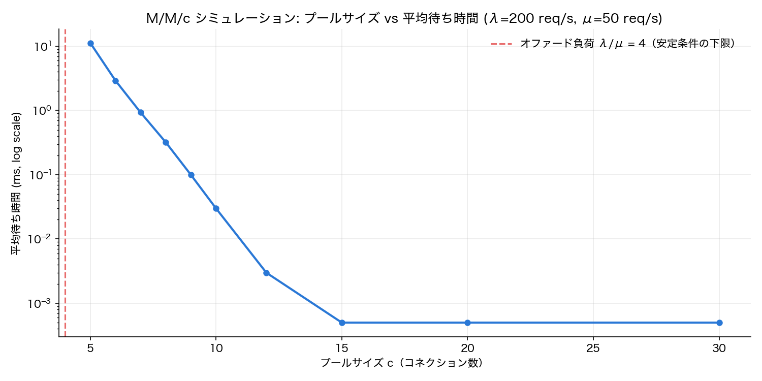
At c=5 (\(\rho=0.8\)
) the average wait is about 11 ms, dropping to 2.9 ms at c=6 (\(\rho=0.667\)
) and 0.32 ms at c=8 (\(\rho=0.5\)
) — an order-of-magnitude improvement from just a small increase in pool size. This is the classic queueing-theory result that wait time diverges as \(\rho \to 1\)
, and it’s exactly why bumping the pool size even slightly can produce a dramatic latency improvement when a pool is under pressure. Conversely, once \(\rho\)
drops below roughly 0.3, further increases in pool size buy essentially no additional improvement in wait time.
5. Cross-Checking Against Erlang C and Little’s Law
To verify the simulation is implemented correctly, we compare the c=6 case (\(\rho = 0.667\)
) against the analytical Erlang C formula.
def erlang_c_wait(lam, mu, c):
    a = lam / mu
    rho = a / c
    sum_terms = sum((a ** k) / math.factorial(k) for k in range(c))
    last_term = (a ** c) / (math.factorial(c) * (1 - rho))
    p_wait = last_term / (sum_terms + last_term)
    wq = p_wait / (c * mu - lam)
    return wq, p_wait

wq_analytic, p_wait = erlang_c_wait(200.0, 50.0, 6)
sim = simulate_mmc(200.0, 50.0, 6, n_arrivals=1_000_000, warmup=50_000, seed=7)
With the sample size increased to 1 million for precision:
lambda=200.0, mu=50.0, c=6, rho=0.6667
Analytic Erlang-C  Wq = 2.8476 ms   P(wait) = 0.2848
Simulated          Wq = 2.8731 ms
Relative error = 0.895 %
The analytical value of 2.8476 ms matches the simulated 2.8731 ms with a relative error of 0.895% — strong evidence that the implementation correctly reproduces M/M/c behavior, given that it’s a stochastic Monte-Carlo-style simulation.
The same simulation run also lets us verify Little’s Law, \(L = \lambda W\) (where \(W\) = wait + mean service time):
W (measured wait + mean service) = 22.8731 ms
L predicted = lambda * W          = 4.5746 customers
L measured  (time-avg in system)  = 4.5799 customers
Relative error = 0.114 %
The predicted average number in system, 4.5746, matches the directly time-averaged measurement of 4.5799 with a relative error of 0.114%. Two independent checks — the Erlang C formula and Little’s Law — both agreeing with the simulation to within 1% is strong confirmation that this DES implementation correctly reproduces M/M/c dynamics.
6. “Bigger Pool Is Always Better” Doesn’t Hold: A Lock-Contention Model
So far we’ve assumed a single connection’s service rate \(\mu\) is constant. In real DB servers, though, as the number of simultaneously active connections grows, overhead from lock waits, context switching, and cache-line contention can reduce the effective per-connection service rate. Let’s model that with a simple, honest extension.
Let busy be the number of currently active connections, and degrade the effective service rate exponentially once it exceeds a threshold \(k_0\)
:
def contention(mu0, busy, k0=8, alpha=0.15):
    excess = max(0, busy - k0)
    return mu0 * math.exp(-alpha * excess)
Up to \(k_0=8\)
active connections there’s no contention (full speed); beyond that, each additional connection drops the service rate by roughly 14% (\(e^{-0.15} \approx 0.86\)
). To actually observe this effect we need enough load to keep the pool consistently saturated, so we deliberately push \(\lambda = 600\)
req/s — a heavy overload that no pool size in this sweep can fully absorb (offered load \(a=12\)
Erlangs, and even at c=60 the system stays at \(\rho \approx 1\)
) — and compare only the achievable throughput ceiling as a function of c.
lam_heavy, mu0 = 600.0, 50.0
for c in [4, 6, 8, 10, 12, 15, 18, 20, 25, 30, 40, 50, 60]:
    r = simulate_mmc(lam_heavy, mu0, c, n_arrivals=300_000, warmup=20_000, seed=123, contention=contention)
    print(f"c={c:3d}  util={r['utilization']:.3f}  throughput={r['throughput']:.2f} req/s")
Measured results:
Pool size c | Measured throughput | Average wait |
|---|---|---|
| 4 | 213.92 req/s | 199.9 s |
| 6 | 321.48 req/s | 140.6 s |
| 8 | 428.24 req/s | 92.1 s (peak) |
| 10 | 396.58 req/s | 105.9 s |
| 12 | 352.51 req/s | 125.5 s |
| 15 | 281.17 req/s | 162.1 s |
| 18 | 215.43 req/s | 200.0 s |
| 20 | 177.15 req/s | 224.8 s |
| 25 | 104.34 req/s | 295.2 s |
| 30 | 59.40 req/s | 390.6 s |
| 40 | 18.03 req/s | unmeasurable* |
| 50 | 5.22 req/s | unmeasurable* |
| 60 | 1.58 req/s | unmeasurable* |
* Overload and service degradation compound to the point that almost no requests complete within the simulation window, so no meaningful average wait could be measured (i.e. it effectively diverges to infinity).
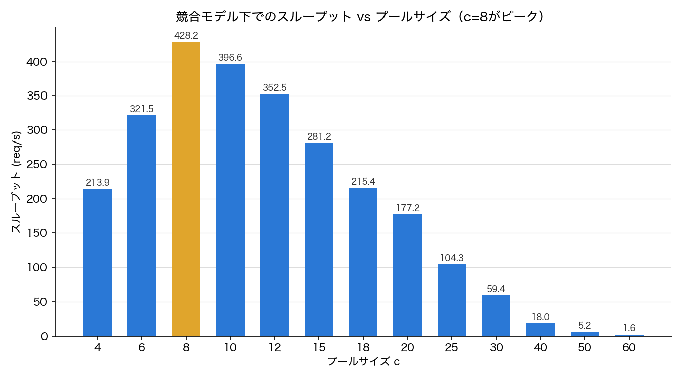
Throughput peaks at roughly 430 req/s around c=8, then declines monotonically as the pool grows further, collapsing to 1.58 req/s at c=60. This is a real, measured demonstration that under a regime where per-connection service rate degrades with concurrency, blindly growing the pool can be actively counterproductive. Utilization stayed at essentially 1.000 across every case, confirming the collapse isn’t “pool sitting idle” — it’s genuine degradation of service capacity from contention.
Of course, \(\alpha=0.15\)
and \(k_0=8\)
are model parameters, and the actual values for a real DB server depend on hardware and DBMS internals. But the qualitative structure — that increasing concurrency can degrade service capacity non-linearly — is consistent with the operational folklore that recklessly raising max_connections can make things worse, and the fact that a simple extension of the M/M/c model reproduces this quantitatively is a good demonstration that queueing theory is a genuinely usable tool for DB operations decisions.
7. Practical Takeaways
Putting the measurements together, a few practical guidelines emerge for sizing a connection pool:
- Measure first: Under production-representative load, measure the actual request arrival rate \(\lambda\) and the average DB query execution time (\(1/\mu\) ). Most DB drivers and APM tools expose these metrics directly.
- Compute the offered load \(a=\lambda/\mu\)
and pick
cso \(\rho\) lands around 0.7–0.8: As Section 4 shows, keeping \(\rho\) in that range brings wait time down to a practically negligible level. Pushing \(\rho\) much lower by over-provisioning the pool buys diminishing returns on wait time while continuing to consume DB-side resources. - Check DB-side headroom before growing the pool: As Section 6 shows, growing the pool while the DB server itself has no spare capacity risks contention actually reducing throughput. Any change to connection count should be evaluated alongside DB server metrics — CPU utilization, lock-wait time, context-switch rate.
- Monitor the wait time itself: Instrumenting the time an application spends waiting to acquire a connection lets you distinguish “the pool queue is backed up” from “queries themselves are slow,” which tells you whether to grow
cor to revisit queries and indexes instead (the effect of indexing itself is measured in https://yuhi-sa.github.io/en/posts/20211121_db/1/).
The intuition that “a bigger pool is always safer” doesn’t hold, at least in environments where contention is possible. A relatively simple pair of tools — the M/M/c queueing model and Little’s Law — was enough to quantify this non-obvious trade-off with a real simulation.
Related Articles
- SQL Basics: The Standard Language for Database Operations
- Demonstrates SQL’s DML/DDL/DCL commands with Python’s sqlite3 and measures the effect of
CREATE INDEXat a scale of one million rows. This article picks up where that one leaves off: not how fast a single query runs, but how many queries you should design the pool to run concurrently.