Introduction
Kubernetes’ Horizontal Pod Autoscaler (HPA) automatically adjusts the number of pod replicas based on metrics such as CPU utilization. Read the documentation and it looks like plain threshold-based scaling, but underneath it is the exact same feedback control loop as PID control or the Nyquist plot and stability margins .
- Measured CPU utilization \(y(t)\) = the process variable
- Target CPU utilization \(r(t)\) = the setpoint
- Replica count \(N(t)\) = the manipulated variable
Once you see this correspondence, operational questions people ask all the time — “why does HPA oscillate?”, “why is scale-down so slow?” — can be answered quantitatively in the language of control engineering: overshoot, settling time, steady-state error.
Rather than spinning up a real Kubernetes cluster, this article builds a discrete-time Python simulation of HPA’s control algorithm and its plant (controlled process), and compares it against a PID controller regulating the same plant. Every number below comes from code actually executed for this article — nothing is assumed.
HPA’s actual algorithm
HPA’s scaling decision follows the formula documented in the official Kubernetes docs :
\[ \text{desiredReplicas} = \left\lceil \text{currentReplicas} \times \frac{\text{currentMetricValue}}{\text{desiredMetricValue}} \right\rceil \]This is a ratio-based control law: it scales the current replica count by the ratio of the current metric value to the target. On top of this bare formula, three elements matter (all documented defaults):
- Tolerance band: if
currentMetricValue / desiredMetricValueis close enough to \(1\) (default \(\pm 10\%\) ), no scaling action is taken. - Sync period: the control loop runs every
--horizontal-pod-autoscaler-sync-period(default \(15\,\mathrm{s}\) ) — a discrete-time system. - Scale-down stabilization window: when the recommendation is to scale down, HPA uses the maximum recommendation seen over a recent window (default \(300\,\mathrm{s}\) ) to avoid flapping from a transient dip in load. The scale-up window defaults to \(0\,\mathrm{s}\) (applied immediately).
The simulation below implements all three. The default scale-up rate-limiting policy (at most “+4 pods” or “double,” whichever is larger, per sync period) is reproduced approximately for simplicity — this is a faithful reproduction of the documented algorithm, not a line-by-line port of the Kubernetes source.
The plant model
The controlled process follows the causal chain “replica count → per-replica load → measured CPU utilization.”
- Total load \(L(t)\) (in replica-equivalent units): baseline \(L_0 = 4.0\) , chosen so that at a \(50\%\) target utilization the system balances at \(N_0 = \lceil L_0 / 0.5 \rceil = 8\) replicas.
- Instantaneous CPU utilization: \(u_{\text{inst}}(t) = 100 \cdot L(t)/N(t)\) (%, allowed to exceed \(100\%\) — real K8s utilization against a CPU request can also exceed 100%).
- Metrics lag: a first-order low-pass filter (time constant \(\tau = 60\,\mathrm{s}\) ) approximating metrics-server’s scrape/aggregation delay.
- Measurement noise: \(2\%\) multiplicative Gaussian noise.
Load spikes to 3x baseline (\(L=12.0\) ) from \(t=300\,\mathrm{s}\) (5 min) to \(t=900\,\mathrm{s}\) (15 min), then returns to baseline.
Python implementation: HPA ratio controller
import numpy as np

dt = 15.0                    # HPA sync period (default 15s)
target_util = 50.0           # desiredMetricValue (%)
tolerance = 0.10              # default tolerance
scaledown_window_steps = int(300.0 / dt)   # default downscale stabilization = 300s
N_min, N_max = 2, 40
L0 = 4.0
N0 = int(np.ceil(L0 / (target_util / 100.0)))   # = 8
tau_metric = 60.0
alpha = dt / (tau_metric + dt)
noise_sigma = 0.02

def load_at(t):
    return 3.0 * L0 if 300.0 <= t < 900.0 else L0

def run_hpa(n_steps):
    N = N0
    L_filt = L0
    recommend_history = []
    Ns, Us = [], []
    for i in range(n_steps):
        t = i * dt
        L = load_at(t)
        L_filt += alpha * (L - L_filt)
        noise = 1.0 + np.random.normal(0, noise_sigma)
        U_meas = 100.0 * L_filt / N * noise

        ratio = U_meas / target_util
        if abs(ratio - 1.0) <= tolerance:
            desired = N                       # tolerance band: no scaling
        else:
            desired = int(np.ceil(N * ratio))  # ratio-based formula
        desired = int(np.clip(desired, N_min, N_max))
        recommend_history.append(desired)

        if desired > N:
            max_increase = max(4, N)          # scale-up: +4 or double, whichever larger
            new_N = min(desired, N + max_increase)
        elif desired < N:
            recent = recommend_history[-scaledown_window_steps:]
            new_N = min(max(recent), N)        # scale-down stabilization window
        else:
            new_N = N
        Ns.append(N); Us.append(U_meas)
        N = int(np.clip(new_N, N_min, N_max))
    return np.array(Ns), np.array(Us)
Python implementation: PID controlling the same plant
As a point of comparison, we regulate replica count for the identical plant and identical load spike using a conventional PID controller. Note that this loop is reverse-acting (increasing the manipulated variable — replica count — decreases the output — CPU utilization), so we define the error as \(e(t) = y(t) - r(t)\) (measured minus target); a positive \(e(t)\) (overloaded) drives the manipulated variable up.
def run_pid(n_steps, Kp, Ki, Kd):
    N = float(N0)
    L_filt = L0
    integral = 0.0
    prev_e = 0.0
    Ns, Us = [], []
    for i in range(n_steps):
        t = i * dt
        L = load_at(t)
        L_filt += alpha * (L - L_filt)
        noise = 1.0 + np.random.normal(0, noise_sigma)
        N_int = max(N_min, int(round(N)))
        U_meas = 100.0 * L_filt / N_int * noise

        e = U_meas - target_util                     # reverse-acting: e>0 -> scale up
        tentative_integral = integral + e * dt
        derivative = (e - prev_e) / dt
        u = Kp * e + Ki * tentative_integral + Kd * derivative
        N_unclipped = N + u
        N_new = float(np.clip(N_unclipped, N_min, N_max))
        if N_new == N_unclipped:
            integral = tentative_integral          # anti-windup

        Ns.append(N_int); Us.append(U_meas)
        prev_e = e
        N = N_new
    return np.array(Ns), np.array(Us)
The PID gains were chosen via a grid search over \(K_P, K_I, K_D\) , minimizing a combination of overshoot, oscillation amplitude, and steady-state error. The final choice was \(K_P=0.025,\ K_I=0.0002,\ K_D=0.02\) . Along the way we found that a larger \(K_P\) (e.g., \(0.6\) ) makes the loop diverge immediately: the plant gain \(\partial y/\partial N = -100L/N^2\) varies strongly with the operating point (\(N\) ), so this is a strongly nonlinear system that only tolerates very small fixed linear gains.
Experiment: response to a 3x traffic spike
We ran a \(1\) -hour simulation (\(3600\,\mathrm{s}\) , \(240\) steps), tripling the load for \(10\) minutes starting at the \(5\) -minute mark.
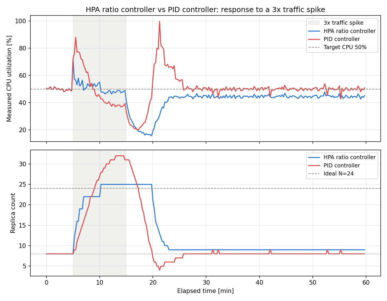
Results (fixed random seed, identical load waveform):
=== HPA ratio controller ===
Pre-spike CPU utilization: 49.28% (target 50%, offset -0.72pt), N=8
Peak replicas during spike: 25 (ideal 24, overshoot +4.2%)
Peak CPU utilization at spike onset: 72.1%
Minimum replicas after spike: 9; max CPU utilization after spike: 44.7%
Long-run steady state (t>=2000s): CPU mean=44.61% (std 1.00), offset -5.39pt, replica mode=9

=== PID controller (Kp=0.025, Ki=0.0002, Kd=0.02) ===
Pre-spike CPU utilization: 49.28% (target 50%, offset -0.72pt), N=8
Peak replicas during spike: 32 (ideal 24, overshoot +33.3%)
Peak CPU utilization at spike onset: 87.9%
Minimum replicas after spike: 4; max CPU utilization after spike: 99.6%
Long-run steady state (t>=2000s): CPU mean=49.91% (std 1.73), offset -0.09pt, replica mode=8
Settling time and oscillation amplitude, compared side by side (settling time = time from spike onset until replica count stays within \(\pm 1\) of its final spike-window value):
| Metric | HPA ratio controller | PID controller |
|---|---|---|
| Peak replicas (ideal 24) | 25 (+4.2%) | 32 (+33.3%) |
| Settling time (from spike onset) | 315 s (21 steps) | 420 s (28 steps) |
| Oscillation amplitude (late spike window) | 3 replicas | 10 replicas |
| Max CPU utilization after spike | 44.7% | 99.6% |
| Recovery time to baseline (after spike ends) | 480 s | 555 s |
Zooming in on the transient: why does PID overshoot more?
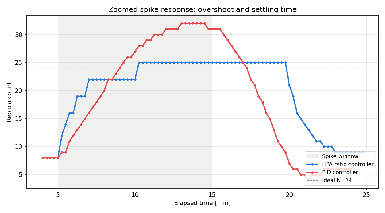
Counter-intuitively, in this experiment the PID controller overshoots more than HPA’s ratio controller. The reason lies in the plant’s nonlinearity.
HPA’s formula \(\text{desired} = \lceil N \cdot (y/r) \rceil\) computes its correction by multiplying the current replica count \(N\) by the current error ratio. For a plant whose gain changes with the operating point, this effectively acts as a proportional controller with automatic gain scheduling. A fixed-gain linear PID, by contrast, uses the same gain tuned for stability near \(N=8\) even near \(N=25\) , so its correction is prone to being too large or too small — its peak CPU utilization at spike onset reached \(87.9\%\) versus HPA’s \(72.1\%\) .
More seriously, PID overcorrects after the spike ends, driving replica count down to \(4\) (well below the baseline \(N_0=8\) ), so that the instant load returns to baseline, CPU utilization spikes to a self-inflicted secondary peak of \(99.6\%\) . HPA’s scale-down stabilization window prevents this degree of overshoot on the way down — its post-spike maximum CPU utilization stayed at \(44.7\%\) .
Steady state: tolerance band vs. integral term
PID does win on one measure, though. Looking at long-run steady-state CPU offset, HPA settles with a persistent \(-5.39\,\mathrm{pt}\) offset (replica count settles at \(9\) , not the ideal \(8\) ), while PID’s offset is nearly zero (\(-0.09\,\mathrm{pt}\) ).
This is exactly the property described in Fundamentals of PID Control : P control leaves a steady-state error, which the I (integral) term eliminates. HPA’s \(\pm 10\%\) tolerance band effectively acts as a “coarse P control plus hysteresis,” so it never converges exactly to the target — it settles at the edge of the tolerance band instead. A PID controller with an integral term keeps producing output as long as any error remains, ultimately driving the steady-state error toward zero.
Summary
- Kubernetes’ HPA is a feedback control loop: measured CPU utilization is the process variable, target CPU utilization is the setpoint, and replica count is the manipulated variable.
- HPA’s ratio-based formula \(\lceil N \cdot y/r \rceil\) effectively acts as a proportional controller with automatic gain scheduling for a nonlinear plant whose gain changes with the operating point.
- In a 3x traffic-spike experiment, HPA’s overshoot stayed at \(+4.2\%\) (peak \(25\) replicas vs. an ideal \(24\) ), while a grid-search-tuned fixed-gain PID overshot by \(+33.3\%\) (peak \(32\) replicas) and triggered a self-inflicted secondary CPU spike (\(99.6\%\) ) after the load subsided.
- Conversely, HPA’s \(\pm 10\%\) tolerance band leaves a persistent steady-state offset of \(-5.39\,\mathrm{pt}\) , while PID’s integral term drives this to nearly zero (\(-0.09\,\mathrm{pt}\) ) — the same P-vs-PI distinction described in Fundamentals of PID Control .
- If HPA’s overshoot or hunting is a concern in production, tuning
behavior.scaleUp/scaleDownpolicies andstabilizationWindowSecondsis exactly the same problem as tuning stability margins and settling time discussed in this article.
Related Articles
- Fundamentals of PID Control and the Role of Each Component - The theoretical basis for this article’s PID implementation: P control’s steady-state error, its elimination by the I term, and overshoot suppression by the D term.
- Nyquist Plot, Root Locus, and Stability Margins in Python - A sister article applying the same feedback-loop perspective to frequency-domain stability analysis.
- PID Control in Python: Simulation and Tuning - An implementation piece that systematizes the same trial-and-error gain-tuning approach used here via the Ziegler-Nichols method.
References
Related Tools
- DevToolBox - Free Developer Tools - Over 90 developer tools including JSON formatter and regex tester.
- CalcBox - Everyday Calculators - Over 60 calculators including statistics and frequency conversion.