Why Static Thresholds Break Down in Server Monitoring
If you’ve monitored servers with Prometheus, you’ve almost certainly written an alert like “fire when CPU usage exceeds 90%.” But production metrics have properties that break this simple approach:
- The baseline itself moves with daily traffic patterns (quiet at night, peak at midday)
- Autocorrelated noise from scrape intervals — noise at one point bleeds into the next scrape
- Both gradual drift (latency slowly worsening from a memory leak) and sudden spikes (transient load bursts) occur in the same metric
A fixed threshold that works at 2am floods you with false alarms at noon, and one tuned for noon misses real degradation at 2am. This is fundamentally a filtering problem. This blog has covered the theory of the EMA filter and the Kalman filter ; this post applies both directly to Prometheus-style anomaly detection, injecting synthetic anomalies into a simulated metric and quantitatively comparing detection performance. The general theory of time-series anomaly detection is covered in Time Series Anomaly Detection: From Statistical Methods to Kalman Filters ; this article focuses specifically on the server-monitoring use case and digs into how parameter tuning affects detection performance.
Two Approaches
Approach 1: EWMA + Adaptive Threshold (Bollinger-band style)
We smooth the metric level with an EMA filter while also tracking the residual variance via EWMA, forming a Bollinger-band-like mean ± kσ adaptive band.
\[ \hat{\mu}_t = (1 - \alpha) \hat{\mu}_{t-1} + \alpha x_t \tag{1} \] \[ \hat{\sigma}^2_t = (1 - \alpha) \hat{\sigma}^2_{t-1} + \alpha (x_t - \hat{\mu}_{t-1})^2 \tag{2} \] \[ \text{alarm}_t = \left| x_t - \hat{\mu}_{t-1} \right| > k \hat{\sigma}_{t-1} \tag{3} \]Here \(\hat{\mu}_{t-1}\) is the level before incorporating the current observation \(x_t\) — this ordering matters, because if you updated the level first, an anomalous value would widen its own band and blunt detection. \(\alpha\) controls smoothing strength and \(k\) controls threshold strictness.
Approach 2: Scalar Kalman Filter (Local-Level Model)
We apply the Kalman filter as a 1D local-level model (a random walk with \(A=1\) plus observation noise).
\[ x_k = x_{k-1} + w_{k-1}, \quad w_{k-1} \sim \mathcal{N}(0, Q) \tag{4} \] \[ z_k = x_k + v_k, \quad v_k \sim \mathcal{N}(0, R) \tag{5} \]With predicted covariance \(P_{k|k-1} = P_{k-1|k-1} + Q\) , innovation \(y_k = z_k - \hat{x}_{k|k-1}\) , and innovation covariance \(S_k = P_{k|k-1} + R\) , we flag anomalies as:
\[ \text{alarm}_k = |y_k| > k \sqrt{S_k} \tag{6} \]Where EWMA smooths level and variance with a single parameter \(\alpha\) , the Kalman filter’s theoretical advantage is that it separates process noise \(Q\) (how much the metric itself can legitimately vary) from observation noise \(R\) (scrape-level measurement noise).
Simulation Design
We generate a synthetic Prometheus-style metric (request latency, ms) with numpy. Assuming a 15-second scrape interval, we generate \(N=2000\) points (about 8.3 hours).
import numpy as np

np.random.seed(42)
N = 2000
t = np.arange(N)

# Baseline: gradual daily traffic variation
baseline = 50 + 8 * np.sin(2 * np.pi * t / N)

# AR(1) autocorrelated noise (simulating scrape-interval correlation)
phi, sigma_e = 0.6, 3.0
noise = np.zeros(N)
for i in range(1, N):
    noise[i] = phi * noise[i - 1] + np.random.randn() * sigma_e

x = baseline + noise
We inject four anomaly types:
| Anomaly | Window (scrape index) | Duration | Scenario |
|---|---|---|---|
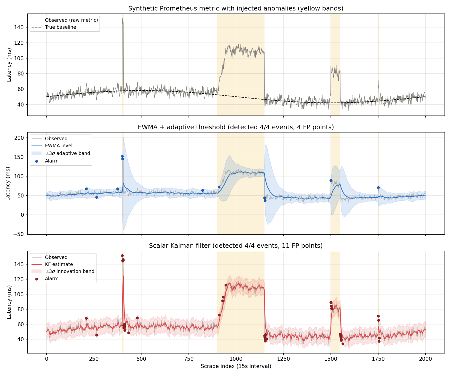
| Spike | [400, 406) | 6 points | Transient load surge (+90ms) |
| Gradual creep | [900, 1150) | 250 points | Memory-leak-like degradation (ramps to +60ms over 50 points, then holds) |
| Step change | [1500, 1550) | 50 points | Deploy-induced regression (+40ms, sudden) |
| Subtle blip | [1750, 1754) | 4 points | Minor anomaly near the noise floor (+22ms) |
These represent plausible real failure modes: the spike and step are sharp transitions that should be easy to catch, the creep is a hard-to-detect gradual change, and the blip sits close to the noise floor.
Detection Results
Both methods ran with EWMA \(\alpha=0.05\) , Kalman filter \(Q=0.5,\ R=9.0\) (matching \(R=\sigma_e^2\) ), and threshold \(k=3\sigma\) .
def evaluate(alarms, anomaly_windows, buffered_mask, n):
    tp_events, latencies = 0, []
    for name, s, e in anomaly_windows:
        window_alarms = np.where(alarms[s:e])[0]
        if len(window_alarms) > 0:
            tp_events += 1
            latencies.append(int(window_alarms[0]))
        else:
            latencies.append(None)
    fp_count = int(np.sum(alarms & ~buffered_mask))
    return tp_events, latencies, fp_count, int(np.sum(alarms))
The results:
| Method | Events detected | FP points | Total alarm points |
|---|---|---|---|
| EWMA + adaptive threshold | 4/4 | 4 | 13 |
| Scalar Kalman filter | 4/4 | 11 | 45 |
Both methods detected all four anomalies, but the Kalman filter’s false-positive count (11) was 2.75x EWMA’s (4). Detection latency (scrape points from event onset to first alarm) matched exactly between the two: the spike, step, and blip were caught instantly (0-point latency), while the creep — due to its gradual ramp — was detected with a 10-point delay in both methods.
Comparing smoothing performance (RMSE against the true baseline): raw data scored 21.94, the EWMA level 20.35, and the KF estimate 21.28 — under AR(1) autocorrelated noise, the two methods’ smoothing performance was nearly identical. This makes sense: EWMA and the local-level-model Kalman filter are mathematically closely related (the steady-state Kalman gain converges to a fixed EWMA-equivalent coefficient). With each method’s parameters individually tuned as in this experiment, most of the performance gap comes not from “which model” but from “how the threshold behaves,” as the next section shows.
Parameter Sensitivity: Push Q Too High and the Filter Starts “Chasing” — and Missing — Real Anomalies
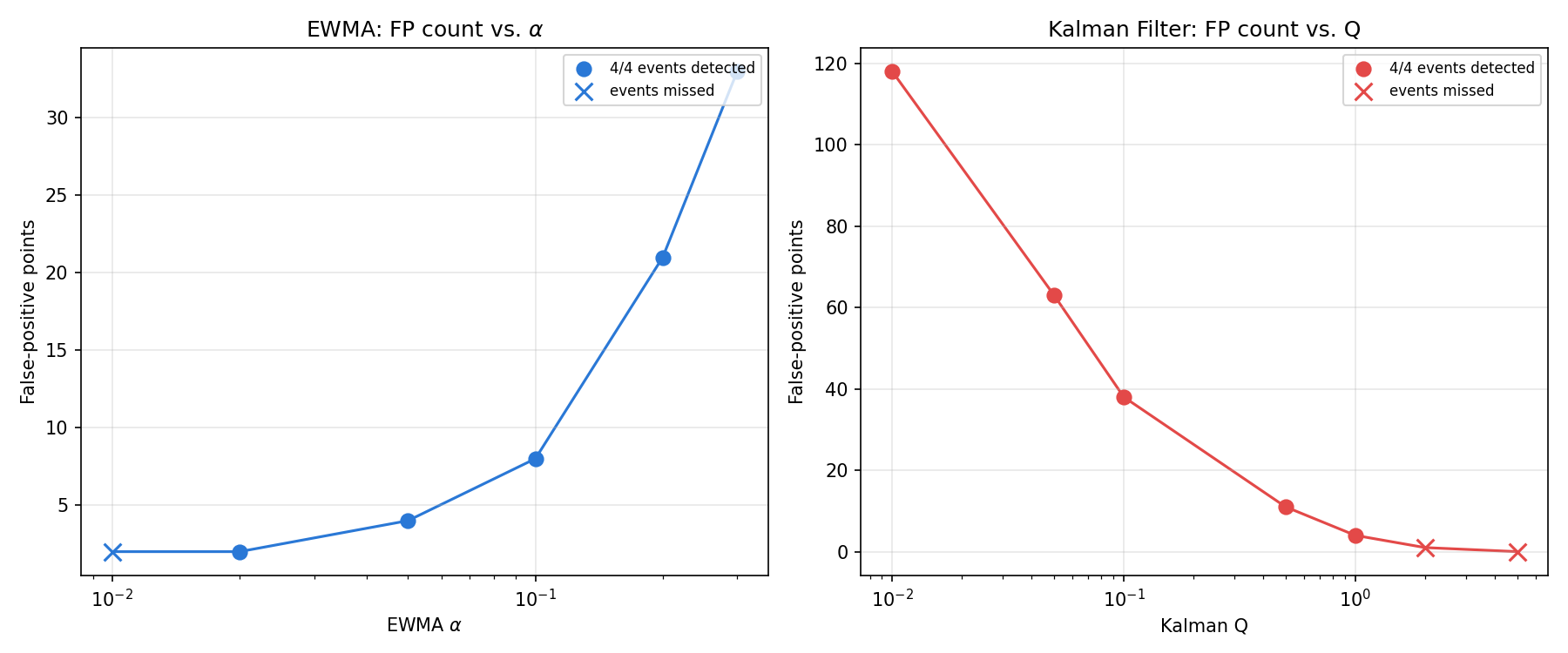
Taken at face value, the results above look like a win for EWMA — but that conclusion depends heavily on parameter choice. We swept EWMA’s \(\alpha\) and the Kalman filter’s \(Q\) (with \(R=9.0\) fixed) to see the detection-rate vs. false-positive tradeoff.
alphas = [0.01, 0.02, 0.05, 0.1, 0.2, 0.3]
for alpha in alphas:
    lvl, var, alarms = ewma_detector(x, alpha=alpha, k=3.0)
    tp, lat, fp, total = evaluate(alarms, anomaly_windows, buffered_mask, N)
    # alpha=0.01 -> 3/4 detected (misses blip), FP=2
    # alpha=0.05 -> 4/4 detected, FP=4
    # alpha=0.30 -> 4/4 detected, FP=33 (too sensitive, FP explodes)

Qs = [0.01, 0.05, 0.1, 0.5, 1.0, 2.0, 5.0]
for Q in Qs:
    est, istd, alarms = kalman_detector(x, Q=Q, R=9.0, k=3.0)
    tp, lat, fp, total = evaluate(alarms, anomaly_windows, buffered_mask, N)
    # Q=0.01 -> 4/4 detected but FP=118 (band too narrow, reacts to noise)
    # Q=1.0  -> 4/4 detected, FP=4 (matches EWMA's best case)
    # Q=2.0, 5.0 -> 3/4 detected (misses creep)
The full sweep:
EWMA (\(\alpha\) sensitivity):
| \(\alpha\) | Detected | FP points | Missed event |
|---|---|---|---|
| 0.01 | 3/4 | 2 | blip |
| 0.02 | 4/4 | 2 | none |
| 0.05 | 4/4 | 4 | none |
| 0.10 | 4/4 | 8 | none |
| 0.20 | 4/4 | 21 | none |
| 0.30 | 4/4 | 33 | none |
Kalman filter (\(Q\) sensitivity, \(R=9.0\) fixed):
| \(Q\) | Detected | FP points | Missed event |
|---|---|---|---|
| 0.01 | 4/4 | 118 | none |
| 0.05 | 4/4 | 63 | none |
| 0.10 | 4/4 | 38 | none |
| 0.50 | 4/4 | 11 | none |
| 1.00 | 4/4 | 4 | none |
| 2.00 | 3/4 | 1 | creep |
| 5.00 | 3/4 | 0 | creep |
Two operationally important findings fall out of this:
- Raising \(Q\) (or \(\alpha\) ) reduces false positives, but past a point the filter starts missing the gradual creep anomaly. At \(Q \geq 2.0\) , the memory-leak-like creep event could no longer be detected. A larger \(Q\) makes the filter track observations more aggressively, so it absorbs a slow degradation as if it were a legitimate level shift. This produces a paradox: the exact class of anomaly you most want to catch — a slowly worsening failure — gets missed precisely at the settings that look best by false-positive count alone.
- The Kalman filter can match EWMA’s best-case false-positive rate (FP=4) once tuned to \(Q=1.0\) , but getting there required moving \(Q\) over two orders of magnitude (0.01 → 1.0). EWMA reached a comparably good balance already around \(\alpha=0.02\) . In terms of tuning effort, EWMA was the easier method to work with in this experiment.
So the question “which is better, EWMA or Kalman filter?” turns out to reduce less to the model itself and more to how forgiving each is to tune, and what pitfalls its parameters hide — a conclusion this simulation lets us state with actual numbers rather than intuition.
Wiring This Into Prometheus (Sketch)
The core of this article is the Python-side validation, but here’s a rough sketch of production wiring:
- Use a recording rule with
deriv()oravg_over_time()to precompute an EWMA-equivalent smoothed series as a separate metric - Express the threshold check in an Alertmanager rule, e.g. something like
abs(raw - smoothed) > k * stddev_over_time(...) - The Kalman filter needs sequential state updates that PromQL alone can’t express well; in practice this means running the filter in a sidecar or exporter and exporting its estimate and confidence interval back to Prometheus as separate metrics
Either way, the conclusion stands: the alerting threshold \(k\) and the model parameter (\(\alpha\) or \(Q\) ) both need tuning to match the failure mode you care about (sharp vs. gradual).
Summary
- Static thresholds are a poor fit for Prometheus metrics with daily seasonality; an EWMA adaptive threshold or Kalman-filter innovation-based check both work better
- In this simulation both methods detected all four injected anomalies, but with each tuned near reasonable defaults, the Kalman filter’s false-positive count was 2.75x EWMA’s — this is a snapshot at particular parameter choices, not a general ranking
- Pushing the Kalman filter’s \(Q\) too high causes the model to track and absorb gradual anomalies (memory-leak-like creep) instead of flagging them — a real pitfall that’s easy to fall into if you tune purely by minimizing false positives
- EWMA reached a good detection/false-positive balance with less parameter search, making it the more forgiving method to operate in this experiment
Monitoring data — noisy and non-stationary by nature — rewards understanding the underlying filtering theory ( EMA , Kalman filter ) and validating parameter sensitivity against real data, rather than trusting either method’s defaults blindly.
Related Articles
- Frequency Characteristics of the Exponential Moving Average (EMA) Filter - The EMA filter theory and frequency response underlying this post’s adaptive threshold.
- Kalman Filter Theory and Python Implementation - The general form (state-space model, predict/update steps) of the scalar Kalman filter used here.
- Time Series Anomaly Detection: From Statistical Methods to Kalman Filters - A systematic overview of anomaly detection methods (including point vs. interval anomaly taxonomy); this post applies that framework specifically to Prometheus monitoring data.
- Fundamentals of Filtering Methods in Signal Processing - A systematic overview of the Kalman filter, EKF, UKF, and particle filter.
References
- Roberts, S.W. (1959). “Control Chart Tests Based on Geometric Moving Averages.” Technometrics.
- Welch, G., & Bishop, G. (2006). “An Introduction to the Kalman Filter.” UNC Chapel Hill TR 95-041.
- Prometheus Documentation: Recording Rules