1. What Is a Bloom Filter
A Bloom filter is, in one sentence, a probabilistic set-membership data structure with an asymmetric guarantee: it can say “definitely not in the set” with certainty, but its “probably in the set” answer can sometimes be wrong. It answers whether an element belongs to a set without storing a single one of the actual elements — just a small, fixed-size bit array.
This asymmetry is not a bug; it is the design itself. A Bloom filter never produces a false negative, while allowing a certain probability of a false positive. If it says “not present,” you can trust that 100%; if it says “present,” it will be wrong some fraction of the time. Turning this property to your advantage — using it as a fast pre-filter before an expensive real lookup — is the canonical use case.
The structure was invented by Burton H. Bloom, who introduced it in his 1970 paper in Communications of the ACM, “ Space/Time Trade-offs in Hash Coding with Allowable Errors ” ( PDF ). As the title suggests, the motivation was to trade a certain amount of “allowable error” for large savings in time and space in hash coding. More than half a century later, this idea is still very much alive inside distributed databases, search engines, and CDNs.
2. The Mechanism: A Bit Array and k Hash Functions
The core of a Bloom filter is nothing more than a bit array of size \(m\) (initialized to all zeros) together with \(k\) independent hash functions \(h_1, h_2, \dots, h_k\) , each of which returns an integer in \([0, m-1]\) .
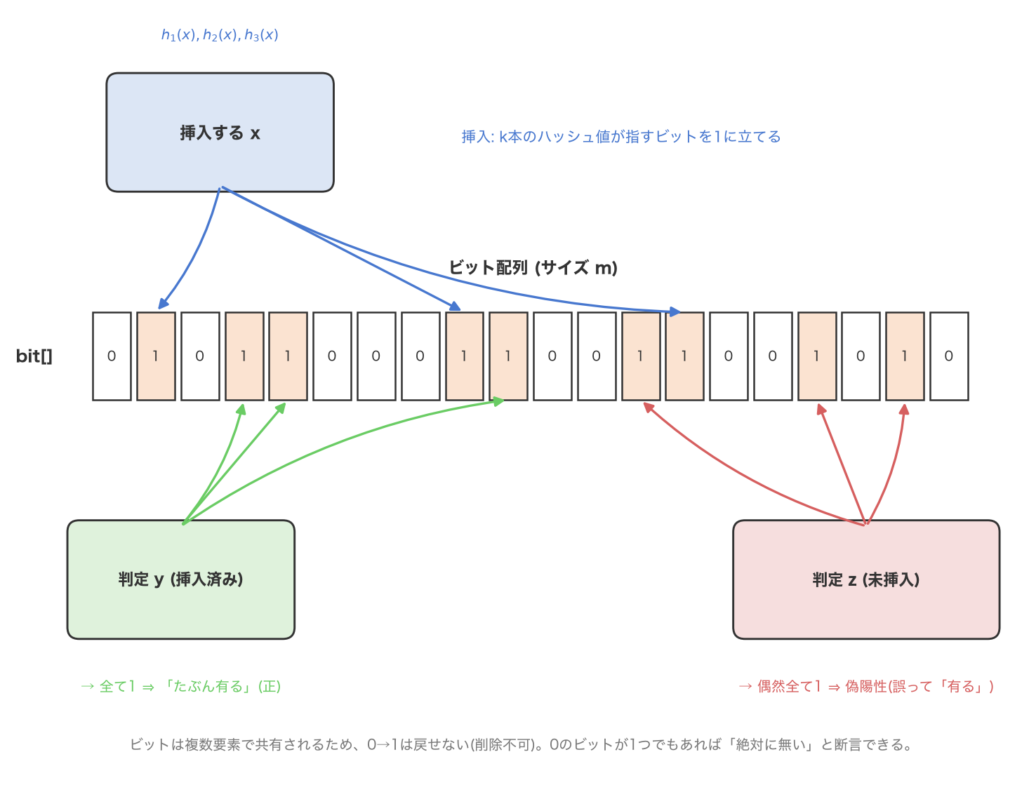
Insert: To insert element \(x\) , compute \(h_i(x)\) for each of the \(k\) hash functions and set all \(k\) corresponding bits to 1.
Query: To test whether element \(y\) is a member, compute \(h_1(y), \dots, h_k(y)\) the same way and inspect the \(k\) corresponding bits.
- If even one bit is 0, \(y\) was definitely never inserted (whatever element set that bit to 1 never included \(y\) , and no bit ever goes back to 0).
- If all \(k\) bits are 1, the filter reports “probably present.” However, \(y\) itself may never have been inserted at all — it’s possible that the insertion of several other elements happened to set all \(k\) of the bits that \(y\) ’s hashes point to. That is exactly a false positive.
The figure below illustrates this. The query for \(y\) (actually inserted) follows three arrows that all point to bits that are 1, so it’s correctly judged “present.” The query for \(z\) (never inserted) also happens to point to three bits that are all 1 — purely by coincidence — and is incorrectly judged “present” as well.
Why Deletion Isn’t Possible
A standard Bloom filter has no delete operation. The reason is simple: a single bit is shared by multiple elements. If you wanted to delete an element by clearing the bits it points to back to 0, you would also erase information belonging to any other element that happens to share one of those bits — causing an element that should still be a member to be incorrectly reported as absent (a false negative, which is strictly worse than a false positive, since it violates the filter’s core guarantee). Setting a bit to 1 is an irreversible operation, and this is the Bloom filter’s single biggest constraint. Section 8 discusses how this constraint is worked around in practice.
3. Deriving the False-Positive Rate
The single most important practical metric for a Bloom filter is its false-positive rate \(p\) . Let’s derive it step by step, assuming ideal random hashing.
After inserting \(n\) elements, focus on one particular bit. A single hash computation selects that bit with probability \(1/m\) , so it is not selected with probability \(1-1/m\) . Since each of the \(n\) elements uses \(k\) hash functions, the total number of hash computations performed during insertion is \(kn\) . So the probability that a given bit is never selected — remains 0 — is
\[ \left(1 - \frac{1}{m}\right)^{kn} \]Using the well-known limit \(\left(1-\frac{1}{m}\right)^{m} \to e^{-1}\) as \(m \to \infty\) , we can approximate this as
\[ \left(1 - \frac{1}{m}\right)^{kn} = \left[\left(1 - \frac{1}{m}\right)^{m}\right]^{kn/m} \approx e^{-kn/m} \]That is, the probability a given bit is still 0 is \(\approx e^{-kn/m}\) , and the probability it is 1 is \(\approx 1 - e^{-kn/m}\) .
A false positive occurs for a never-inserted element \(z\) when all \(k\) of its hashes happen to land on bits that are already 1. Treating the outcomes of the \(k\) hashes as independent (an approximation), multiplying these probabilities together gives the standard approximation for the false-positive rate:
\[ p \approx \left(1 - e^{-kn/m}\right)^{k} \](The exact form without the limit approximation is \(p = \left(1-(1-\frac{1}{m})^{kn}\right)^{k}\) ; for sufficiently large \(m\) the two are nearly identical. Section 5’s experiment compares measured values against both.)
Deriving the Optimal Number of Hash Functions \(k\)
For fixed \(m\) and \(n\) , there is a value of \(k\) that minimizes \(p\) . Let \(x = kn/m\) , so \(p(x) = (1-e^{-x})^{xm/n}\) . Differentiating \(\ln p\) with respect to \(x\) and setting it to zero gives
\[ \ln(1-e^{-x}) + \frac{x\,e^{-x}}{1-e^{-x}} = 0 \]Substituting \(u = e^{-x}\) (so \(x = -\ln u\) ) turns this into
\[ \ln(1-u) - \frac{u \ln u}{1-u} = 0 \]which is satisfied at \(u = 1/2\) , since \(\ln(1/2) - \frac{(1/2)(-\ln 2)}{1/2} = -\ln 2 + \ln 2 = 0\) . So the optimum is \(e^{-x^*} = 1/2\) , i.e. \(x^* = kn/m = \ln 2\) , giving the optimal number of hash functions
\[ k^{*} = \frac{m}{n}\ln 2 \approx 0.6931 \cdot \frac{m}{n} \]Substituting \(e^{-x^*} = 1/2\) back gives the minimum achievable false-positive rate directly:
\[ p^{*} = \left(1-\frac{1}{2}\right)^{k^{*}} = 2^{-k^{*}} \approx 0.6185^{\,m/n} \]a remarkably clean result. In other words, once you decide how many bits per element to allocate (\(m/n\) ), both the optimal number of hash functions and the resulting floor on the false-positive rate are uniquely determined. The next section implements this and checks whether real measurements agree.
4. Python Implementation
Below is a from-scratch numpy implementation. The bit array is represented as a numpy.bool array (one byte per bit), and the hash function is the standard library’s hashlib.blake2b, salted. Rather than computing \(k\)
independent hashes from scratch every time, this implementation uses the Kirsch–Mitzenmacher double-hashing technique: computing just two independent hash values \(h_1, h_2\)
per key is enough to simulate \(k\)
hash functions via the linear combination
This is a technique with solid theoretical backing and wide practical adoption (it’s used, for example, in Guava’s BloomFilter). Thanks to this trick, sweeping dozens of combinations of \(k\)
and bit-array size \(m\)
only requires computing blake2b once per key; the rest is pure numpy vector arithmetic.
import hashlib
import math
import numpy as np

SALT = b"bloom-filter-blog-20260720"

def base_hashes(keys):
    """Compute h1, h2 (64-bit ints) from a blake2b digest for each key (bytes)."""
    h1 = np.empty(len(keys), dtype=np.uint64)
    h2 = np.empty(len(keys), dtype=np.uint64)
    for i, k in enumerate(keys):
        d = hashlib.blake2b(k, salt=SALT[:16], digest_size=16).digest()
        h1[i] = int.from_bytes(d[:8], "little")
        h2[i] = int.from_bytes(d[8:], "little")
    return h1, h2

class BloomFilter:
    """An m-bit, k-hash Bloom filter. Takes precomputed h1, h2 arrays."""

    def __init__(self, m):
        self.m = m
        self.bits = np.zeros(m, dtype=bool)

    def _indices(self, h1, h2, k):
        m = np.uint64(self.m)
        return [((h1 + np.uint64(i) * h2) % m).astype(np.int64) for i in range(k)]

    def insert_all(self, h1, h2, k):
        for idx in self._indices(h1, h2, k):
            self.bits[idx] = True

    def query_all(self, h1, h2, k):
        """True for each key iff all k of its bits are set (filter says "present")."""
        present = np.ones(len(h1), dtype=bool)
        for idx in self._indices(h1, h2, k):
            present &= self.bits[idx]
        return present

def theoretical_fp(k, n, m):
    return (1 - math.exp(-k * n / m)) ** k
insert_all/query_all don’t loop element by element; they take arrays of hash values for every element (or every query) at once and set/read bits in bulk via numpy fancy indexing. This makes it feasible to run dozens of experiments at \(n=100{,}000\)
-element scale — sweeping both bit-array size \(m\)
and hash count \(k\)
— in a reasonable amount of time.
5. Experiment 1: Does Theory Match Measurement?
We verify how accurate the theoretical formula \(p \approx (1-e^{-kn/m})^k\)
actually is on real data. We inserted \(n=100{,}000\)
elements and prepared \(100{,}000\)
never-inserted query keys (with a fixed random seed, generated from mutually disjoint namespaces member-{i} / nonmember-{i} so they can never collide by construction), then measured the false-positive rate for every combination of hash count \(k \in \{2,4,6,8\}\)
and bit ratio \(m/n \in \{4,6,8,10,12,16,20\}\)
.
A sample of the results:
| k | m/n | Measured FP rate | Theoretical \((1-e^{-kn/m})^k\) | Relative error |
|---|---|---|---|---|
| 2 | 8 | 0.047330 | 0.048929 | 3.27% |
| 4 | 8 | 0.023580 | 0.023969 | 1.62% |
| 6 | 10 | 0.008780 | 0.008436 | 4.08% |
| 8 | 12 | 0.003060 | 0.003142 | 2.62% |
| 4 | 20 | 0.001020 | 0.001080 | 5.53% |
Across all 28 combinations, most points show a relative error under 5%. The points that look like outliers (e.g. \(k=6, m/n=20\) : measured 0.000430 vs. theoretical 0.000303, a 41.85% relative error) occur where the theoretical expected number of false positives is tiny — only about 30 out of 100,000 — so Poisson-noise-scale fluctuations (\(\sqrt{30}\approx5.5\) ) are more than enough to explain the gap between the expected ~30 and the observed 43. In other words, the seemingly large errors aren’t the formula failing; they’re simply statistical noise becoming relatively more visible when the event itself is rare.
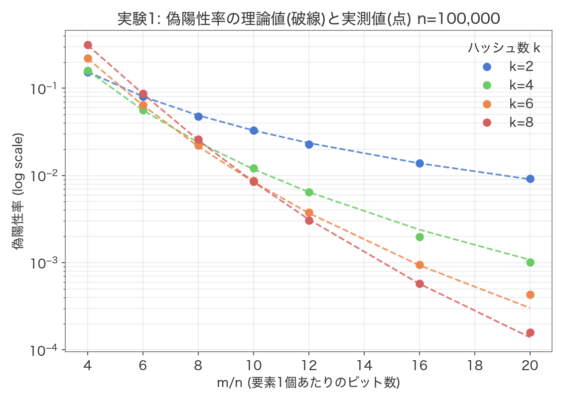
As the figure shows, the theoretical curves and measured points overlap almost perfectly on a log scale, confirming that the limit approximation \(p \approx (1-e^{-kn/m})^k\) is accurate enough for practical use.
6. Experiment 2: Measuring the Optimal Number of Hash Functions k
Next we check whether the optimal hash count \(k^{*} = \frac{m}{n}\ln 2\) derived in Section 3 actually holds up empirically. We fixed \(m/n=10\) (10 bits per element) — so \(m=1{,}000{,}000\) bits for \(n=100{,}000\) — and swept the hash count \(k\) from 1 to 10, measuring the false-positive rate at each. The theoretical optimum here is \(k^{*} = 10 \times \ln 2 = 6.931\) .
| k | Measured FP rate | Theoretical |
|---|---|---|
| 1 | 0.09572 | 0.09516 |
| 2 | 0.03303 | 0.03286 |
| 3 | 0.01805 | 0.01741 |
| 4 | 0.01210 | 0.01181 |
| 5 | 0.01023 | 0.00943 |
| 6 | 0.00878 | 0.00844 |
| 7 | 0.00852 | 0.00819 |
| 8 | 0.00852 | 0.00846 |
| 9 | 0.00930 | 0.00913 |
| 10 | 0.01036 | 0.01019 |
The measured values tie exactly at \(k=7\) and \(k=8\) , both at 852 false positives out of 100,000 — the minimum at this measurement resolution. Rounding the theoretical optimum \(k^{*}=6.931\) gives exactly 7, which matches the measured minimum (7-8) precisely.
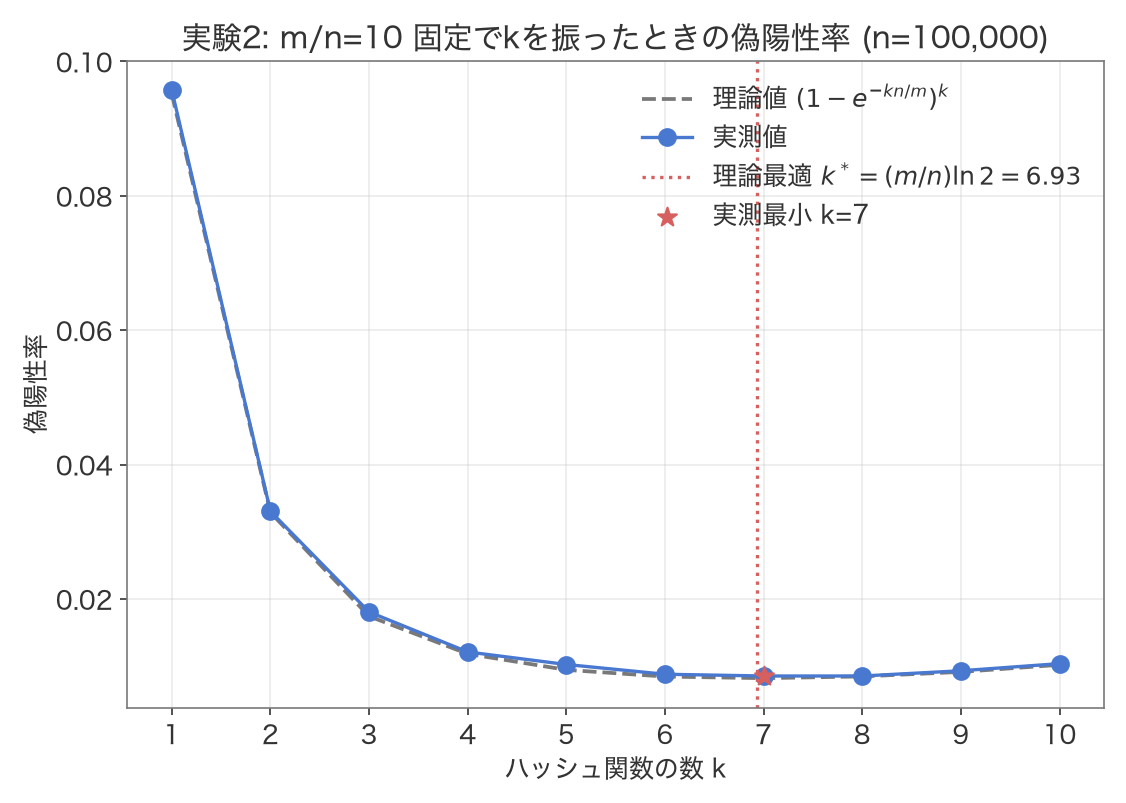
As the U-shaped curve shows, when \(k\) is too small there aren’t enough bits being set to discriminate well; when \(k\) is too large, each insertion sets so many bits at once that the array fills up too quickly. This experiment confirms empirically that the bottom of that trade-off curve sits right where theory predicts, at \(k \approx (m/n)\ln 2\) .
7. Design Cheat Sheet: Deriving m and k from n Elements and a Target False-Positive Rate p
In practice, what you actually want to know when designing a Bloom filter is: given “\(n\) elements” and “an acceptable false-positive rate \(p\) ,” what bit-array size \(m\) and hash count \(k\) do you need? Rearranging Section 3’s results \(p^{*} = 2^{-k^{*}}\) and \(k^{*}=\frac{m}{n}\ln2\) in terms of \(n\) and \(p\) gives the design formula
\[ m = -\frac{n \ln p}{(\ln 2)^2}, \qquad k = \frac{m}{n}\ln 2 \]Here’s a cheat sheet by target false-positive rate:
| Target FP rate \(p\) | Bits needed (per element) | Optimal hash count \(k\) |
|---|---|---|
| 10% | ≈4.8 bits | 3 |
| 5% | ≈6.2 bits | 4 |
| 2% | ≈8.1 bits | 6 |
| 1% | ≈9.6 bits | 7 |
| 0.1% | ≈14.4 bits | 10 |
| 0.01% | ≈19.2 bits | 13 |
For example, to achieve a false-positive rate of 1% or lower over 100 million keys, you need about \(9.6 \times 10^8\) bits (roughly 115 MB) and 7 hash functions — a design you can compute in seconds. Compared to storing the actual data for each key (tens to hundreds of bytes each) in a database or cache, needing just over one byte per element is the essence of a Bloom filter’s space efficiency.
8. How Bloom Filters Are Used in Real Systems
Bloom filters aren’t just an academic curiosity — they’re actively used inside major databases and infrastructure today.
Skipping SSTables in LSM-tree databases: LSM-tree-based databases like Cassandra and RocksDB buffer writes in an in-memory memtable, then flush it to disk as an immutable SSTable file. When reading a key, you don’t know in advance which SSTable holds it, so in the worst case you’d have to open every single SSTable to check. This is exactly where a Bloom filter helps. According to
Cassandra’s official documentation
, each SSTable carries a Bloom filter over its own key set, stored off-heap as the SSTable’s Filter component, with bloom_filter_fp_chance (default 0.01-0.1, depending on the compaction strategy) tunable per table. If a filter says “definitely not in this SSTable,” the disk I/O is skipped entirely, making lookups for non-existent keys dramatically faster.
RocksDB’s Bloom filter implementation
follows the same idea, defaulting to about 10 bits/key per SST file — which, per the cheat sheet in Section 7, corresponds to roughly a 1% false-positive rate.
CDN “one-hit-wonder” detection: Akamai’s CDN found that a striking 75% of cached assets were “one-hit wonders” — requested exactly once and never again. In response, they used a Bloom filter to track whether a given URL had ever been requested before, only promoting an object into the cache on its second request. This keeps content that will never be looked at again from wasting cache capacity, substantially increasing the cache’s effective capacity.
Milvus’s delete filtering: The vector database Milvus also avoids immediate physical deletion, instead recording deletes as a delta log, and uses a Bloom filter at query time to quickly narrow down whether a segment contains any deleted primary keys. Details are covered in our deep dive into Milvus’s internal architecture, /posts/20260719_milvus_internals/1/ (Japanese only).
Derived data structures: Because plain Bloom filters can’t support deletion, several derived structures are widely used to address that limitation. A Counting Bloom Filter replaces each bit with a small counter (typically 4 bits), incrementing on insert and decrementing on delete, at the cost of several times more memory than a plain bit array. A more recent structure, the Cuckoo Filter, stores a short fingerprint of each element in a cuckoo-hashed table rather than setting bits; deletion is as simple as removing one fingerprint, and it’s known to be more space-efficient than a plain Bloom filter when the target false-positive rate is below roughly 3%.
Contrast with cardinality estimation: A sibling probabilistic data structure built from the same ingredients — a hash function and a fixed-size array — is HyperLogLog. It answers a different question, though: where a Bloom filter answers “is this element in the set? (membership),” HyperLogLog estimates “how many distinct elements are in this set? (cardinality)” using \(m\) registers combined via a harmonic mean. See our HyperLogLog deep dive , which verifies the theoretical standard error \(1.04/\sqrt{m}\) against measurement.
Conclusion
A Bloom filter uses an extremely simple pair of ingredients — an \(m\) -bit array and \(k\) hash functions — to guarantee “definitely not present” while cheaply answering “possibly present.” Its false-positive rate is well approximated by \(p \approx (1-e^{-kn/m})^k\) , minimized at \(p^{*}=2^{-k^{*}}\) when the hash count is \(k^{*}=\frac{m}{n}\ln2\) . Our from-scratch numpy implementation confirmed this formula holds within about 5% relative error on real measurements, and that the optimal hash count empirically bottoms out at 7-8, right where the theoretical value of 6.93 predicts. From skipping SSTables to CDN cache admission to filtering deletes in a vector database, Bloom filters are a foundational technique quietly underpinning the performance of many real systems, and worth keeping in your design toolkit.
FAQ
Q1. Can false negatives occur (an inserted element incorrectly reported as “not present”)? No. As long as no delete operation is performed, a bit set during insertion never reverts to 0, so querying a truly-inserted element will always find all \(k\) of its bits set to 1. Under ideal hash functions and a correct implementation, a Bloom filter never produces a false negative, by construction.
Q2. What if I need to delete an element? A plain bit-array Bloom filter has no support for deletion (see Section 2). If deletion is required, the standard approach is to use a Counting Bloom Filter (counters instead of bits) or a fingerprint-based Cuckoo Filter. Periodically rebuilding the entire filter from scratch is another workable option.
Q3. Do I really need \(k\) separate hash functions? In theory, yes — \(k\) independent hash functions. In practice, the Kirsch–Mitzenmacher double-hashing trick from Section 4 lets you compute just two independent hash values and reproduce the effect of \(k\) hashes via the linear combination \(h_i(x)=(h_1(x)+i\cdot h_2(x)) \bmod m\) . This has almost no impact on the theoretical false-positive rate and is the standard approach used in practice.
Q4. When should I use a Bloom filter versus a hash table? A hash table stores the key itself (or enough information about it), so it never produces false positives, but it requires memory roughly proportional to the number of elements — several to tens of bytes each. A Bloom filter needs only about 1-2 bytes per element, in exchange for accepting some false positives. The typical pattern is to use a Bloom filter as a fast pre-filter in front of the real data store (an on-disk SSTable, a database over the network, etc.), leaving the actual existence check to the hash table or real data store behind it.
We’ve also rounded up other field-defining classics in 10 Technical Books Every Engineer Should Read .