1. What’s Wrong with Plain hash(key) mod N
When you want to distribute data or requests across multiple servers, the first idea that comes to mind is usually hash(key) mod N: hash the key and take the remainder modulo the number of servers N. It’s a one-line implementation, and as long as the key distribution is uniform, the assignment across servers is uniform too.
But this approach has one flaw that can be fatal in production: the moment the server count N changes, almost every key’s assigned server changes with it. hash(key) mod 10 and hash(key) mod 11 return completely different remainders for the same hash(key) in almost all cases. For a cache server, the hit rate collapses to near zero instantly; for a distributed database, it triggers a massive physical data migration (resharding). Adding or losing a single server effectively means near-total system churn — an unacceptable cost in modern distributed systems where scaling in and out is routine.
Let’s measure this collapse directly. I measured, over 100,000 keys, the fraction of keys whose assigned server changes under hash(key) mod N when going from a 10-node configuration to an 11-node configuration.
import hashlib

def h64(data: bytes) -> int:
    """Returns the first 8 bytes of a blake2b digest as an unsigned 64-bit integer."""
    d = hashlib.blake2b(data, digest_size=8).digest()
    return int.from_bytes(d, "little")

def mod_assignment(keys, n_nodes):
    return [h64(k) % n_nodes for k in keys]

keys = [f"key-20260720-{i}".encode() for i in range(100_000)]
before = mod_assignment(keys, 10)
after = mod_assignment(keys, 11)
moved = sum(1 for b, a in zip(before, after) if b != a)
print(moved, moved / len(keys))
The measured result:
| Condition | Keys moved | Ratio | Theoretical value |
|---|---|---|---|
10 → 11 nodes (mod N) | 90,899 / 100,000 | 90.90% | approx. \(1-\frac{1}{11}\approx 90.91\%\) |
Over 90% of the 100,000 keys — more than 9 out of every 10 — end up on a different server. This is not a coincidence or an implementation bug; it is a mathematical necessity of the mod N scheme. If the hash values are uniform, only about \(1/11\)
of keys keep the same remainder and stay put, and the remaining \(1-1/11\approx90.9\%\)
must move somewhere. The measured 90.90% matches the theoretical 90.91% almost exactly, confirming that this collapse happens exactly as theory predicts.
Consistent hashing, the subject of this article, was devised to eliminate this “the cache or the sharded data nearly dies every time the server count changes” flaw. The concept was first formalized by David Karger and colleagues in their 1997 STOC (ACM Symposium on Theory of Computing) paper, “ Consistent Hashing and Random Trees: Distributed Caching Protocols for Relieving Hot Spots on the World Wide Web ” (Karger, Lehman, Leighton, Levine, Lewin, Panigrahy, STOC 1997). It was originally proposed as a theoretical framework for relieving web-cache hot spots, but it has since become deeply embedded in the infrastructure layer of modern distributed systems — memcached’s distributed clients, DynamoDB, Cassandra, and the Envoy/HAProxy load balancers among them.
2. How Consistent Hashing Works: The Ring and Clockwise Assignment
The core idea of consistent hashing is simple. Instead of the unstable “remainder modulo server count” mapping, place both nodes and keys on the same circular hash space (a ring), and assign each key to the first node encountered while walking clockwise from the key’s position.
The concrete procedure is as follows.
- Treat the output range of a hash function (e.g. \([0, 2^{64})\) ) as a circle whose two ends are joined.
- Hash each node’s (server’s) identifier, and use that value as its position on the ring.
- Hash each key the same way to get its position on the same ring.
- Starting from the key’s position, search clockwise and assign the key to the first node found.
The figure below shows a ring with nodes A/B/C/D, and a new node E being added.
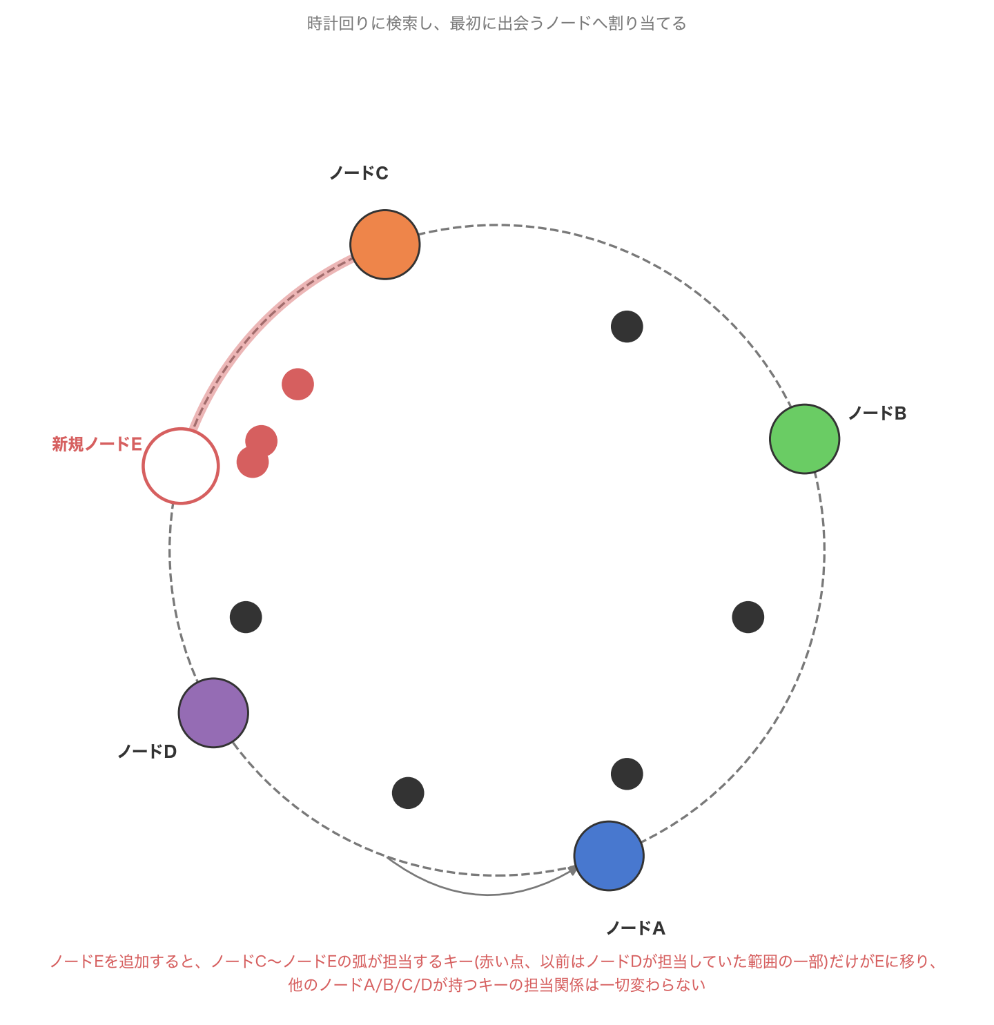
This is the decisive difference from mod N. Adding node E only moves the keys on the arc from the node immediately preceding E (node C in this diagram) to E; every other key’s assignment is completely unchanged. This is intuitive once you notice that no node other than E has moved on the ring. Removing a node is symmetric: only the range it owned is absorbed by the next node on the ring, with no effect on any other node.
This locality — that adding or removing a node only affects its immediate neighborhood on the ring — is the essence of consistent hashing. As the phrase “Random Trees” in Karger’s paper title suggests, placing nodes randomly on the ring is shown theoretically to yield two properties simultaneously: for n nodes, every node’s expected share of the ring is about \(1/n\)
, and the impact of any change is localized.
3. Experiment: Is Remapping Really Limited to About \(1/n\) ?
In theory, when going from 10 nodes to 11, the fraction of keys the new node takes over should equal its share of the ring (about \(1/11\) of the whole), while the other 10 nodes’ ranges stay unchanged. That gives a theoretical remapping ratio of \(1/11\approx9.09\%\) . I verified this against the same 100,000 keys and the same random seed used in Section 1.
import bisect

class HashRing:
    """A simple blake2b-based consistent hash ring. Supports a virtual-node count v."""

    def __init__(self, node_ids, v=1):
        self.v = v
        self.ring_points = []  # list of (position, node_id), sorted ascending by position
        for node_id in node_ids:
            for vi in range(v):
                pos = h64(f"{node_id}#{vi}".encode())
                self.ring_points.append((pos, node_id))
        self.ring_points.sort(key=lambda t: t[0])
        self.positions = [p for p, _ in self.ring_points]

    def lookup(self, key: bytes) -> str:
        pos = h64(key)
        idx = bisect.bisect_right(self.positions, pos)
        if idx == len(self.positions):
            idx = 0  # wrap around to the start of the ring
        return self.ring_points[idx][1]

nodes10 = [f"node-{i}" for i in range(10)]
nodes11 = [f"node-{i}" for i in range(11)]
ring_before = HashRing(nodes10, v=200)  # 200 virtual nodes, matching ketama's typical range
ring_after = HashRing(nodes11, v=200)

before = [ring_before.lookup(k) for k in keys]
after = [ring_after.lookup(k) for k in keys]
moved = sum(1 for b, a in zip(before, after) if b != a)
print(moved, moved / len(keys))
The measured result:
| Condition | Keys moved | Ratio | Theoretical value |
|---|---|---|---|
| 10 → 11 nodes (consistent hashing, v=200) | 9,106 / 100,000 | 9.11% | approx. \(1/11\approx 9.09\%\) |
The measured 9.11% matches the theoretical 9.09% to within 0.02 percentage points. Compared to mod N moving 90.90% of keys, the same “10 → 11 nodes” change moves roughly one-tenth as many keys under consistent hashing. The chart below places both side by side.
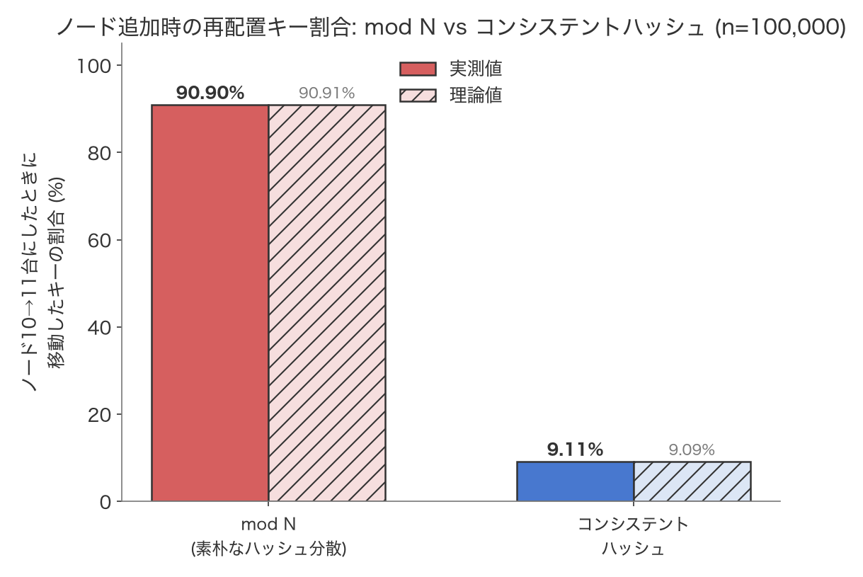
In general, going from n nodes to n+1, the fraction of keys consistent hashing moves is about \(1/(n+1)\)
— the more nodes there already are, the smaller the impact of adding one more. Conversely, when n is small the moved fraction is proportionally larger, but it always stays vastly smaller than mod N’s \(1-1/(n+1)\)
. This property — that the impact of a change is localized in inverse proportion to the node count — is precisely why consistent hashing became the standard technique behind distributed caches and databases.
4. Load Imbalance and Virtual Nodes
The ring built for the experiments above used v=200 virtual nodes. A virtual node means placing one physical node not at a single point on the ring, but at multiple points (each hashed separately with a suffix like #0, #1, …). Why is this necessary? Trying v=1 (no virtual nodes — one point per physical node) shows why immediately.
Placing physical nodes at just one random point each on the ring makes the gaps between nodes purely random, so the gap sizes (and hence the ranges each node owns) can vary wildly — a large-range node next to a small-range one. This is exactly the elementary problem of “how much do the gaps between 10 randomly placed points on a circle vary” — and with few points, the imbalance can be severe.
With 10 nodes and 100,000 keys, I swept the virtual-node count \(v \in \{1, 10, 100, 1000\}\) and measured the coefficient of variation (CV = standard deviation / mean) of the key count each node received. A smaller CV means a more even load.
import statistics

nodes = [f"node-{i}" for i in range(10)]
for v in [1, 10, 100, 1000]:
    ring = HashRing(nodes, v=v)
    counts = {node: 0 for node in nodes}
    for k in keys:
        counts[ring.lookup(k)] += 1
    values = list(counts.values())
    mean = statistics.mean(values)
    cv = statistics.pstdev(values) / mean
    print(v, mean, cv, min(values), max(values))
The measured result (mean is 10,000 keys/node across the 10 nodes):
| Virtual nodes \(v\) | CV (stdev/mean) | Min keys | Max keys |
|---|---|---|---|
| 1 | 0.9415 | 910 | 32,508 |
| 10 | 0.3821 | 5,251 | 18,485 |
| 100 | 0.0575 | 9,095 | 11,038 |
| 1,000 | 0.0279 | 9,545 | 10,382 |
At \(v=1\) , despite an average of 10,000 keys/node, the least-loaded node got only 910 keys while the most-loaded got 32,508 — over three times the average — and the CV of 0.94 is enormous. This completely undermines the expectation that “spreading across 10 nodes cuts the load to one-tenth.” As \(v\) increases to 10, 100, and 1,000, the CV shrinks rapidly to 0.38, 0.058, and 0.028, and by \(v=1000\) the gap between min and max is under 10%.
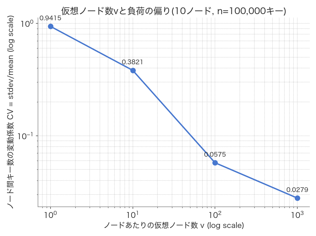
As the figure shows, CV decreases almost monotonically with the logarithm of \(v\) . Virtual nodes can be understood as scattering each physical node “thinly and widely” across many points on the ring, averaging out the randomness of the gaps by a law-of-large-numbers effect. The property from Section 3 — that remapping stays around \(1/n\) — holds even without virtual nodes, but the practically important property that each node’s load is roughly even only reaches a usable level once enough virtual nodes are in place. These are two distinct properties that resemble each other, and this experiment let us separate and measure them independently.
5. Python Implementation (Full Code)
Consolidating everything used so far into one piece of code:
import bisect
import hashlib
import statistics


def h64(data: bytes) -> int:
    """Returns the first 8 bytes of a blake2b digest as an unsigned 64-bit integer."""
    d = hashlib.blake2b(data, digest_size=8).digest()
    return int.from_bytes(d, "little")


class HashRing:
    """A simple blake2b-based consistent hash ring. Supports a virtual-node count v."""

    def __init__(self, node_ids, v=1):
        self.v = v
        self.ring_points = []
        for node_id in node_ids:
            for vi in range(v):
                pos = h64(f"{node_id}#{vi}".encode())
                self.ring_points.append((pos, node_id))
        self.ring_points.sort(key=lambda t: t[0])
        self.positions = [p for p, _ in self.ring_points]

    def lookup(self, key: bytes) -> str:
        pos = h64(key)
        idx = bisect.bisect_right(self.positions, pos)
        if idx == len(self.positions):
            idx = 0
        return self.ring_points[idx][1]

    def lookup_many(self, keys):
        return [self.lookup(k) for k in keys]


def mod_assignment(keys, n_nodes):
    return [h64(k) % n_nodes for k in keys]


def remap_ratio(before, after):
    moved = sum(1 for b, a in zip(before, after) if b != a)
    return moved, moved / len(before)


def load_cv(ring, node_ids, keys):
    counts = {node: 0 for node in node_ids}
    for k in keys:
        counts[ring.lookup(k)] += 1
    values = list(counts.values())
    mean = statistics.mean(values)
    return statistics.pstdev(values) / mean, counts
The HashRing class does everything with just two operations: the constructor places each node at v virtual points on the ring (__init__), and lookup uses bisect_right to find the nearest ring point clockwise from a key’s position. Production libraries typically use a faster hash function (MurmurHash3, xxHash) and a faster ring-lookup structure, but these few dozen lines are enough to reproduce the essential behavior of consistent hashing.
6. Real-World Usage: Dynamo, Cassandra, ketama, Envoy/HAProxy
Consistent hashing is not merely theoretical — it is actively used in major infrastructure today.
Amazon Dynamo (2007): The paper describing Amazon’s internal distributed key-value store Dynamo, “ Dynamo: Amazon’s Highly Available Key-value Store ” (DeCandia et al., SOSP 2007), identifies two problems with plain consistent hashing in Section 4.2: “the random position assignment of each node… leads to non-uniform data and load distribution,” and “the basic algorithm is oblivious to the heterogeneity in the performance of nodes.” Its solution is the virtual node covered in this article. The paper states the benefits as: “if a node becomes unavailable… the load handled by this node is evenly dispersed across the remaining available nodes,” and “when a node becomes available again, or a new node is added… the newly available node accepts a roughly equivalent amount of load from each of the other available nodes.” This design philosophy carries over to the later managed service, DynamoDB.
Cassandra: Per the official Apache Cassandra documentation , single-token consistent hashing makes incremental scaling of small clusters difficult, and Cassandra solves this by assigning multiple tokens (virtual nodes, or vnodes) to each physical node. The default in the 2.x line was 256 tokens per node; from 3.x onward, a more efficient token-allocation algorithm achieves an even balance with fewer tokens.
ketama (memcached): The person who popularized consistent hashing among distributed memcached clients was Richard Jones of Last.fm, who published libketama in 2007. Per that post, prior implementations had the problem that “whenever we added or removed servers from the pool, everything hashed to different servers, which effectively wiped the entire cache.” ketama solves this by hashing each server onto 100–200 points on a continuous circle (“the continuum”), and was released as a C core library with PHP and Java bindings. This “100–200 points per node” figure is the same value later adopted, under the name “ketama,” by Envoy’s ring hash load balancer.
Envoy / HAProxy: The L7 proxy Envoy has a
ring hash (ketama) load balancer
that hashes each host onto a ring and routes requests, hashed on some request property, to the nearest host clockwise. The ring size is tunable via minimum_ring_size (default 1024) and maximum_ring_size (default 8 million), and hosts are placed on the ring proportionally to their weight to support weighting. HAProxy achieves the same kind of consistent hashing by combining balance uri with hash-type consistent, routing the same URI to the same backend repeatedly to boost cache efficiency.
7. Variants: Rendezvous, Jump, and Maglev Hashing
Consistent hashing comes with the overhead of building and maintaining a sorted ring, and several variants exist to avoid that. Rendezvous hashing (HRW: Highest Random Weight), proposed in 1996 by David Thaler and Chinya Ravishankar, dispenses with the ring entirely: for every key-node pair, a “weight” is computed from a hash, and the node with the highest weight is chosen as the owner. Jump Consistent Hash, presented by Google’s John Lamping and Eric Veach in their 2014 paper “ A Fast, Minimal Memory, Consistent Hash Algorithm ,” computes a bucket number with a short loop and no memory at all — but buckets must be numbered sequentially from 0 to n-1, making it unsuitable for freely adding or removing nodes by name. Maglev hashing, used by Google’s software L4 load balancer as described in “ Maglev: A Fast and Reliable Software Network Load Balancer ” (NSDI 2016), divides the hash space into a fixed-length lookup table and constructs it so each backend holds nearly the same number of table slots, achieving even more uniform load balancing and faster lookups than plain consistent hashing.
Summary
Consistent hashing places both nodes and keys on the same circular hash space and assigns each key to the first node encountered walking clockwise — a simple rule that localizes the impact of node-count changes to just the affected neighborhood. In this experiment, going from 10 to 11 nodes remapped 90.90% of keys (theory: 90.91%) under plain mod N, versus 9.11% (theory: 9.09%) under consistent hashing — roughly one-tenth, exactly as theory predicts. I also measured that increasing the virtual-node count from 1 to 1,000 shrinks the coefficient of variation of per-node load from 0.94 to 0.028. The virtual nodes introduced by the Dynamo paper, the 100–200-point continuum popularized by ketama, Cassandra’s 256 tokens, and the ring hash used by Envoy/HAProxy are all extensions of this same “ring plus virtual nodes” combination — proof that a hashing theory nearly half a century old still quietly underpins load distribution in distributed systems today.
FAQ
Q1. How is this different from ordinary hash distribution (mod N)?
mod N theoretically moves nearly all keys (a fraction of \(1-1/N\)
) to a different node whenever the node count N changes. Consistent hashing, by placing nodes and keys on the same ring, limits the moved keys to roughly the difference between the old and new node’s ranges (about \(1/N\)
). The measurements in Sections 1 and 3 (90.90% vs. 9.11%) confirm this gap directly.
Q2. How many virtual nodes are needed? In this experiment, \(v=100\) gave a CV of 0.058, and \(v=1000\) gave 0.028. Both ketama and Envoy use around 100–200 points per node as their standard, which is an empirically well-balanced level — small enough to keep load imbalance practically negligible without making the ring’s memory footprint or lookup cost excessive. If stricter uniformity is required, a dedicated technique like Maglev hashing (Section 7) is worth considering.
Q3. How do you weight nodes? If you’re mixing nodes with different specs, give higher-spec nodes more virtual points on the ring. The Dynamo paper also states that “the number of virtual nodes that a node is responsible for” is decided based on its capacity, accounting for heterogeneity in the physical infrastructure; Envoy’s ring hash load balancer likewise generates ring points proportional to each host’s weight.
Q4. When should you use it? Use it whenever the number of nodes (servers, shards, cache servers) may grow or shrink over time, and you want to avoid massive data migration or total cache invalidation each time it does. This covers backend selection for distributed caches, partitioning for distributed databases, and backend selection in load balancers — anywhere you need “the same key to keep going to roughly the same destination, even as the set of destinations changes dynamically.”
The other domains’ definitive reading lists are collected in 10 Technical Books Every Engineer Should Read .