1. Why Counting Unique Items Is Hard
“How many distinct user IDs appear in this log?” “How many unique visitors did we get today?” These questions look trivial at small scale, but once the data reaches millions or billions of records, they turn into a surprisingly stubborn engineering problem.
There is exactly one way to count exactly: remember every element you have ever seen, and check each new one against that memory. In practice this typically means a hash set (Python’s set, for instance), and this approach comes with an unavoidable memory cost. With \(n\)
elements, a hash set’s memory grows in proportion to \(n\)
. As we’ll measure directly in Section 7, Python’s set consumes on the order of tens to a hundred bytes per element, so exactly counting 100 million unique IDs alone would require several gigabytes of memory.
An even thornier issue is merging across a distributed system. If logs are scattered across dozens of servers and you want the “combined unique count across all of them,” you have to gather every server’s set in one place and take the union. Since the size of a set is exactly the amount of data you’d need to transfer, exact set-based approaches are fundamentally at odds with distributed aggregation.
The approach that trades a small amount of error for a dramatic reduction in memory and network traffic is the probabilistic data structure. Its lineage traces back to the probabilistic counting method introduced by Philippe Flajolet and G. Nigel Martin in their 1985 paper “ Probabilistic Counting Algorithms for Data Base Applications ” (Journal of Computer and System Sciences) — the Flajolet–Martin algorithm. Building on that foundation, and passing through the LogLog algorithm, the 2007 paper “ HyperLogLog: the analysis of a near-optimal cardinality estimation algorithm ” (AofA 2007) by Flajolet, Fusy, Gandouet, and Meunier introduced HyperLogLog (HLL), the subject of this article. With a single pass that does nothing more than hash each element, it achieves a standard error of \(1.04/\sqrt{m}\) using only a fixed amount of memory proportional to the register count \(m\) . This article walks through the theory, builds a from-scratch Python implementation, and checks how closely the measured results track the theoretical predictions.
2. The Intuition: “I Saw a Hash With k Leading Zeros”
At its core, the idea behind HyperLogLog is about as simple as coin-flip probability.
Imagine flipping a fair coin repeatedly and asking about the event “heads comes up \(k\) times in a row.” A single flip comes up heads with probability \(1/2\) , so \(k\) heads in a row happens with probability \(2^{-k}\) . Turning that around: if you actually observe a run of \(k\) heads in a row even once, you must have drawn a fairly rare event — one that happens only about once in every \(2^{k}\) tries.
Now replace coin flips with hash bits. An ideal hash function’s output can be treated as a sequence of independent, roughly fifty-fifty coin flips. If you observe an element whose hash value has \(k\) leading zero bits, that is a rare event with probability around \(2^{-(k+1)}\) , and you can work backward to estimate: “we must have inserted roughly \(2^{k+1}\) unique elements by now.” Since identical elements always hash to the same value, this estimate has the pleasant property of being invariant to duplicates — inserting the same element a thousand times changes nothing.
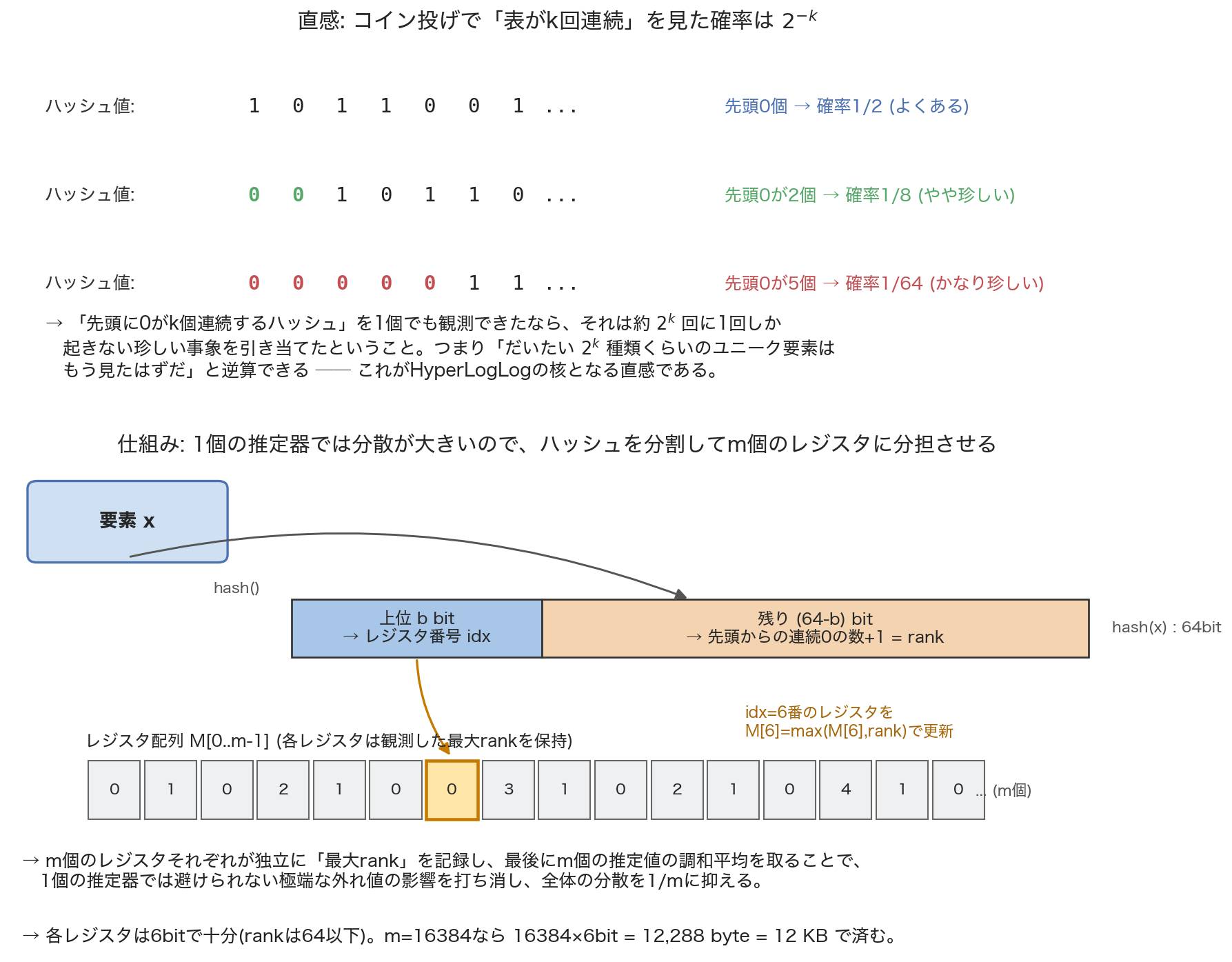
This is, in essence, the original Flajolet–Martin-style algorithm: keep a single register \(R\) (the longest run of leading zeros seen so far), and you can estimate the unique count on the order of \(2^{R}\) . The next section explains why this “single register” approach is unusable as-is.
3. The Variance Problem With a Single Estimator, and m Registers Plus the Harmonic Mean
The estimate from \(R\) in the previous section has a fatal weakness: its variance is far too large. \(R\) is “the maximum seen so far,” and the distribution of a maximum has a long tail (occasionally you draw an extremely large \(R\) purely by chance). Passing that through an exponential function like \(2^R\) means a small wobble in \(R\) can double or quadruple the estimate. It’s like trying to estimate “the probability of heads” by watching a single coin — inherently unstable.
The naive fix is to prepare \(m\) independent hash functions, compute \(m\) values of \(R\) , and average them. But computing \(m\) hash functions every time multiplies the hashing cost by \(m\) , and constructing \(m\) genuinely independent hash functions is a hassle in its own right.
The clever trick in HyperLogLog is to simulate \(m\) independent estimators using a single hash computation (a technique called stochastic averaging). Split the hash’s bit string into two parts:
- The upper \(b\) bits (a value in \(0\) to \(m-1\) , where \(m=2^b\) ) become the register index \(idx\)
- Within the remaining \((64-b)\) bits, compute “the number of consecutive leading zeros, plus one” as the rank
Every time an element is processed, update the register \(idx\) it belongs to with the larger of its current value and this rank (\(M[idx] \leftarrow \max(M[idx], \text{rank})\) ). After processing every element, each of the \(m\) registers independently holds “the maximum run of leading zeros observed” for its own (disjoint) subset of elements. The bottom panel of the figure above illustrates this.
The final piece is the harmonic mean. Computing \(2^{M_j}\) from each register’s value \(M_j\) gives roughly the inverse-scale estimate of “the unique count handled by that register.” If we took a plain arithmetic mean here, a single register that happened to draw an extremely large \(M_j\) would blow up \(2^{M_j}\) and dominate the average. The harmonic mean strongly dampens the influence of large values, giving it strong outlier resistance and pulling the overall variance across the \(m\) registers down to order \(1/m\) . This is precisely why HyperLogLog is designed to take a harmonic mean, and it’s the core reason Flajolet et al. (2007) were able to derive the remarkably small standard error of \(1.04/\sqrt{m}\) .
4. The Estimator Formula, Bias Correction, and Small-Range Linear Counting
Let’s turn the previous section’s idea into math. Given the register array \(M[0..m-1]\) , the raw estimate is computed as
\[ E = \alpha_m \, m^{2} \left( \sum_{j=0}^{m-1} 2^{-M_j} \right)^{-1} \]The quantity \(m\) times the reciprocal of \(\sum_j 2^{-M_j}\) is exactly \(m\) times the harmonic mean of the values \(2^{M_j}\) (by the very definition of the harmonic mean, \(m / \sum_j (2^{M_j})^{-1}\) ) — this is a direct formalization of “estimate the unique count via the harmonic mean,” as described above. \(\alpha_m\) is a bias-correction constant, given by Flajolet et al. (2007) as
\[ \alpha_m = \begin{cases} 0.673 & (m=16) \\ 0.697 & (m=32) \\ 0.709 & (m=64) \\ \dfrac{0.7213}{1+1.079/m} & (m \ge 128) \end{cases} \]This constant corrects a systematic bias inherent to max-based estimators (derived via a Mellin-transform analysis); all the \(m\) values used in this article, \(m=256\) through \(16{,}384\) , fall under the \(m\ge128\) case.
For sufficiently large element counts \(n\) , this estimator achieves a standard error of
\[ \frac{\sigma[E]}{n} \approx \frac{1.04}{\sqrt{m}} \]The crucial point here is that this error does not depend on \(n\) . Whether \(n\) is 100,000 or 100 million, the relative error stays essentially the same as long as \(m\) is fixed. This is exactly why Redis and GA4 (discussed later) can operate with a fixed-size sketch regardless of cardinality.
However, the formula above only works well once \(n\) is reasonably large. If \(n\) is small relative to the register count \(m\) , many registers remain untouched at 0, and \(E\) becomes unstable. To handle this, Flajolet et al. (2007) propose switching to a classic correction called linear counting whenever the raw estimate satisfies \(E \le 2.5m\) :
\[ E^{*} = m \ln\frac{m}{V} \]where \(V\) is the number of registers still at 0. This formula comes from coupon-collector-style statistics — “given \(n\) balls thrown into \(m\) bins, how many bins remain empty” — and covers the regime where \(n\) is small relative to the register count (i.e., where leading zeros almost never occur) with high accuracy. Classic 32-bit-hash implementations also need a correction for cardinalities approaching \(2^{32}\) , but our implementation uses a 64-bit hash, and since \(2^{64}\) is vastly larger than the \(n \le 1{,}000{,}000\) range explored in our experiments, that correction never triggers and is omitted here.
5. Python Implementation
We build a 64-bit integer hash with blake2b, and manage the register array as a bytearray with one byte per register (a rank never exceeds roughly 64, so 6 bits would technically suffice, but we prioritized implementation simplicity).
import hashlib
import math

SALT = b"hyperloglog-blog-20260720"


def hash64(key: bytes) -> int:
    """Compute a 64-bit integer hash via blake2b."""
    d = hashlib.blake2b(key, salt=SALT[:16], digest_size=8).digest()
    return int.from_bytes(d, "big")


def alpha_m(m: int) -> float:
    """Flajolet et al. 2007's bias-correction constant alpha_m (asymptotic formula, m>=128)."""
    return 0.7213 / (1 + 1.079 / m)


class HyperLogLog:
    def __init__(self, b: int):
        """b: number of bits used for the register index. Register count m = 2^b."""
        self.b = b
        self.m = 1 << b
        self.registers = bytearray(self.m)
        self.rem_bits = 64 - b

    def add_hash(self, h: int) -> None:
        """Register a single 64-bit integer hash value."""
        idx = h >> self.rem_bits
        remainder = h & ((1 << self.rem_bits) - 1)
        if remainder == 0:
            rank = self.rem_bits + 1
        else:
            rank = self.rem_bits - remainder.bit_length() + 1
        if rank > self.registers[idx]:
            self.registers[idx] = rank

    def add(self, key: bytes) -> None:
        self.add_hash(hash64(key))

    def raw_estimate(self) -> float:
        m = self.m
        inv_sum = sum(2.0 ** (-r) for r in self.registers)
        return alpha_m(m) * m * m / inv_sum

    def estimate(self) -> float:
        """Estimate including the small-range (linear counting) correction."""
        m = self.m
        e = self.raw_estimate()
        if e <= 2.5 * m:
            zeros = self.registers.count(0)
            if zeros != 0:
                return m * math.log(m / zeros)
            return e
        return e

    def merge(self, other: "HyperLogLog") -> "HyperLogLog":
        """Taking the elementwise max of two register arrays yields the union's HLL."""
        assert self.b == other.b
        out = HyperLogLog(self.b)
        out.registers = bytearray(
            max(a, b) for a, b in zip(self.registers, other.registers)
        )
        return out
idx = h >> self.rem_bits extracts the upper \(b\)
bits of the hash as the register index, and the rank comes from bit_length() of the remaining bits. The simplicity of the merge method — just an elementwise max — is directly responsible for the “strength under distributed aggregation” we measure in Section 7.
6. Experiment 1: Is the Error Determined Solely by the Register Count m?
In theory, the relative standard error is \(1.04/\sqrt{m}\) and shouldn’t depend on the true cardinality \(n\) . Let’s check this empirically.
For each register count \(m \in \{256, 1{,}024, 4{,}096, 16{,}384\}\) (\(b\in\{8,10,12,14\}\) ), we swept the true cardinality \(n\) from \(100{,}000\) to \(1{,}000{,}000\) in steps of 100,000 (10 checkpoints), running 30 trials at each point with a different random seed (elements were unique strings mixed with per-trial random suffixes). We computed the relative error \((E-n)/n\) for every trial and checkpoint, and took the overall RMS (root mean square) across all of them as the “measured relative standard error.”
| \(b\) | \(m\) | Measured RMS relative error | Theoretical \(1.04/\sqrt{m}\) | Mean bias |
|---|---|---|---|---|
| 8 | 256 | 6.858% | 6.500% | +0.480% |
| 10 | 1,024 | 3.638% | 3.250% | -0.325% |
| 12 | 4,096 | 1.675% | 1.625% | +0.228% |
| 14 | 16,384 | 0.744% | 0.813% | +0.082% |
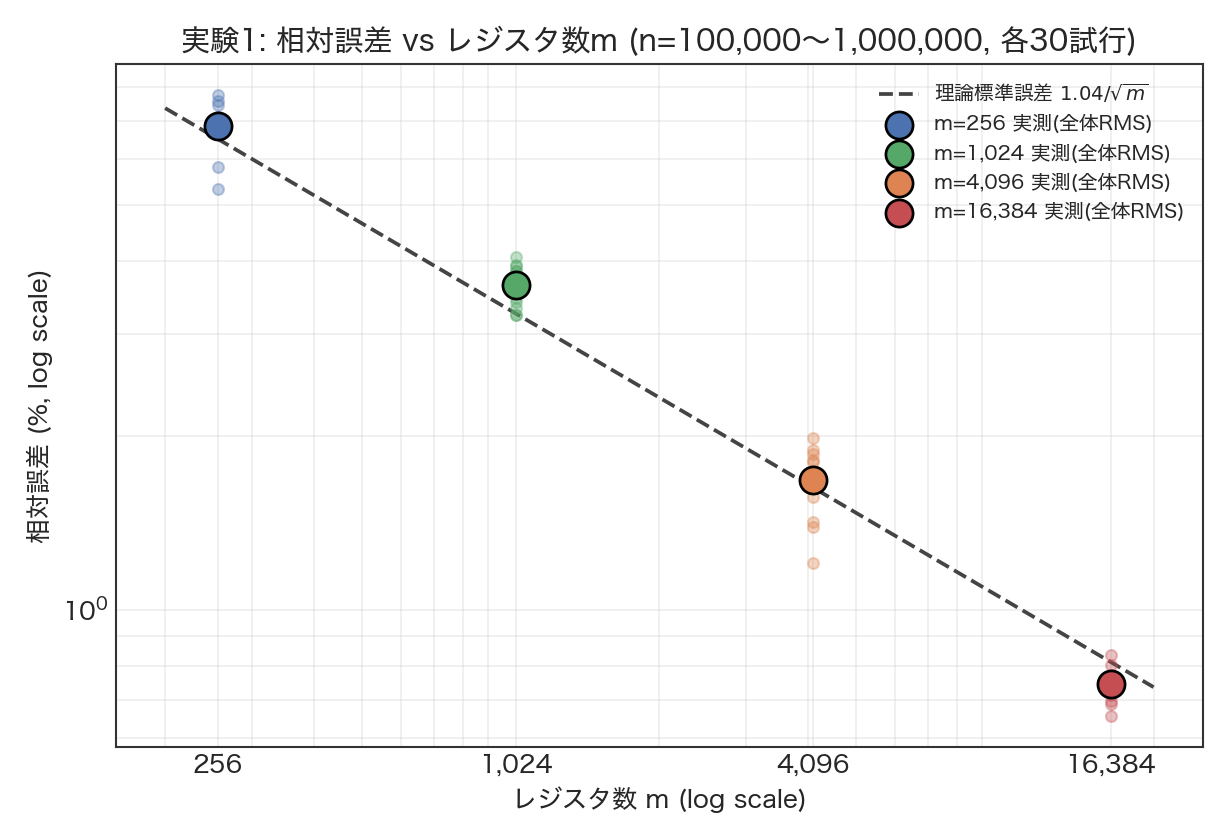
As the figure shows, quadrupling \(m\) roughly halves the error (that is, by \(\sqrt{4}=2\) ), and on a log scale the measured points overlap almost perfectly with the theoretical line. The lightly-plotted per-\(n\) measurements (the 10 points spanning 100,000 to 1,000,000) also cluster at nearly the same level within each \(m\) , confirming empirically that the error is determined by \(m\) alone, independent of \(n\) — exactly as theory predicts. The bias (mean relative error) also stays under 1% in every case, confirming that the \(\alpha_m\) correction is doing its job.
7. Experiment 2: Memory Comparison and Mergeability
Memory Comparison: How Much Smaller Than an Exact Set?
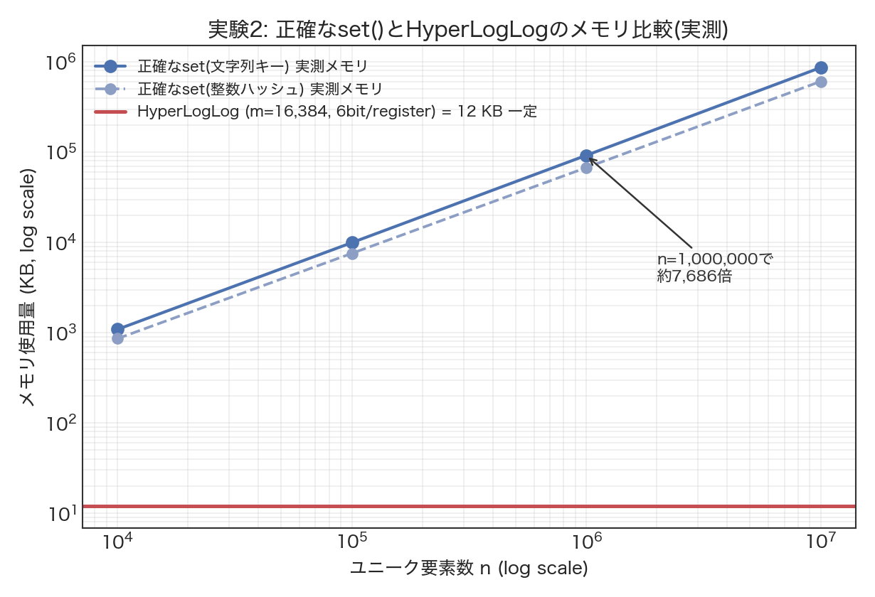
Using tracemalloc, we measured the actual memory consumed as string keys are added to a Python set, and compared it against HyperLogLog’s register array (theoretically \(m \times 6\,\text{bit}\)
; our implementation uses a 1-byte-per-register bytearray for simplicity, though only 6 bits are theoretically needed).
| \(n\) | Measured memory (exact set) | Bytes per element |
|---|---|---|
| 10,000 | 1,087.3 KB | 111.34 B |
| 100,000 | 9,944.7 KB | 101.83 B |
| 1,000,000 | 92,230.0 KB | 94.44 B |
| 10,000,000 | 866,527.9 KB | 88.73 B |
| \(b\) | \(m\) | HyperLogLog register memory |
|---|---|---|
| 8 | 256 | 192 B (0.188 KB) |
| 10 | 1,024 | 768 B (0.750 KB) |
| 12 | 4,096 | 3,072 B (3.000 KB) |
| 14 | 16,384 | 12,288 B (12.000 KB) |
At \(n=1{,}000{,}000\)
, an exact set consumes about 90MB (92,230.0 KB), while a HyperLogLog with \(m=16{,}384\)
needs only 12KB — a gap of roughly 7,686x. And HyperLogLog’s memory stays flat at 12KB no matter how much \(n\)
grows (the red horizontal line in the figure). This is the basis for the “counting unique items in 12KB” in this article’s title — and, as it happens, it’s the exact same value used by Redis’s implementation, discussed below.
Mergeability: Do Two Merged HLLs Land Within the Error Bound?
The single most important property for real-world distributed deployment is mergeability. We built two HyperLogLogs with \(m=16{,}384\)
, with \(|A|=600{,}000\)
, \(|B|=600{,}000\)
, and \(180{,}000\)
shared elements (so the true union size is \(|A\cup B|=1{,}020{,}000\)
). We ran merge — an elementwise max of the register arrays — and computed the union estimate over 10 trials.
| Metric | Value |
|---|---|
| True union size \(\lvert A\cup B\rvert\) | 1,020,000 |
| Mean relative error of merged estimate (10 trials) | +0.089% |
| RMS relative error of merged estimate (10 trials) | 0.536% |
| Theoretical standard error \(1.04/\sqrt{16{,}384}\) | 0.812% |
The merged estimate’s error falls within the theoretical standard error (0.812%), confirming empirically that building HLLs for \(A\) and \(B\) independently and later taking an elementwise max produces (within the error bound) the same result as feeding the entire union \(A\cup B\) into a single HLL from the start. This means each server can build its own local HLL, ship only a 12KB sketch to a central node, and take an elementwise max to recover the global unique count — precisely the distributed aggregation architecture that solves the transfer-cost problem raised in Section 1, where an exact set’s transfer cost scales linearly with element count.
8. How HyperLogLog Is Used in Real Systems
HyperLogLog isn’t just an academic curiosity — it’s actively used throughout large-scale data infrastructure.
Redis PFADD/PFCOUNT/PFMERGE: Redis provides PFADD to add elements to a HyperLogLog, PFCOUNT to retrieve the estimated cardinality, and PFMERGE to union multiple HLLs together. According to
Redis’s official documentation
, the dense representation is “a 12,288-byte string storing 16,384 6-bit counters,” with a stated standard error of 0.81%. That’s the exact same setup as the \(m=16{,}384\)
case we verified in Experiment 2, and it matches the theoretical value \(1.04/\sqrt{16384}\approx0.81\%\)
. At low cardinalities, Redis automatically switches to a sparse representation to save memory further.
BigQuery HLL_COUNT Functions / APPROX_COUNT_DISTINCT:
BigQuery’s HyperLogLog++ function family
uses HLL_COUNT.INIT to build a sketch, HLL_COUNT.MERGE to combine multiple sketches, and HLL_COUNT.EXTRACT to pull out the cardinality. Because a sketch can be stored as a BYTES value in an intermediate table, you can pre-compute sketches per daily partition and later merge any subset of them freely to recompute “unique users over any arbitrary date range.” When precision isn’t specified, APPROX_COUNT_DISTINCT uses the same HLL++ under the hood. What BigQuery calls “precision” corresponds to our \(b\)
(the number of bits used for the register index) — and the trade-off of lower error for higher memory as precision increases is exactly what we confirmed experimentally in Section 6.
Google Analytics 4 (GA4): According to Google’s own explainer on GA4 , GA4 applies HyperLogLog++ with precision 14 (i.e., \(m=16{,}384\) ) for “Active Users” and “Total Users,” and precision 12 (i.e., \(m=4{,}096\) ) for “Sessions.” As it happens, these are exactly the \(m=4{,}096\) and \(m=16{,}384\) cases we verified in Experiments 1 and 2 — and the reason GA4’s dashboard shows user and session counts that aren’t exact figures (except for “new users”) but rather probabilistic estimates is precisely the mechanism we’ve been verifying throughout this article.
Contrast With Bloom Filters: The Bloom filter we covered previously and HyperLogLog here are sibling probabilistic data structures, sharing the same skeleton — a hash function, a fixed-size array, and mergeability. But they answer entirely different questions. A Bloom filter answers “is this element in the set? (yes/no)” — a membership question — with the asymmetric guarantee that false positives can occur but false negatives never do. HyperLogLog answers “how many distinct elements are in this set? (cardinality)” — a counting question — and retains no information whatsoever about any individual element’s presence. In practice the two are often used together rather than as alternatives: for example, using a Bloom filter to pre-filter “have I ever seen this URL before” while HyperLogLog counts the unique URL total in parallel.
Conclusion
HyperLogLog estimates a unique count with a remarkably small standard error of \(1.04/\sqrt{m}\)
, using nothing more than a simple statistic — the longest run of leading zero bits in a hash — spread across \(m\)
registers and combined via a harmonic mean. Across all four values we tested, \(m=256\)
through \(16{,}384\)
, our measured RMS error tracked the theoretical value closely (e.g., at \(m=16{,}384\)
, measured 0.744% versus theoretical 0.813%). Compared to an exact set, it used roughly 7,686x less memory at \(n=1,000,000\)
, and merging two HLLs via an elementwise max produced an estimate that fell within the theoretical error bound. Real-world adoption — Redis’s PFCOUNT (0.81% standard error, 12KB), BigQuery’s HLL_COUNT functions, and GA4’s user and session counts — uses exactly the same \(m\)
values we verified here, showing consistent alignment between theory, implementation, and measurement.
FAQ
Q1. How much error does HyperLogLog have? The standard error is well approximated by \(1.04/\sqrt{m}\) , and (outside the small-range regime) barely depends on the true cardinality \(n\) . For example, \(m=16{,}384\) — Redis’s standard dense representation, and the same setting GA4 uses for user counts — gives roughly 0.81%, while \(m=4{,}096\) gives roughly 1.6%. Experiment 1 confirmed the measured RMS error tracks this theoretical value closely.
Q2. Why use the harmonic mean instead of the arithmetic mean? Computing \(2^{M_j}\) from each register’s value \(M_j\) means a single register that happens to draw an extremely large \(M_j\) can dominate an arithmetic mean, since the underlying distribution has a heavy tail. The harmonic mean strongly dampens the influence of large values, and this outlier resistance is what keeps the overall variance across the \(m\) registers down to order \(1/m\) . This is the core reason Flajolet et al. (2007) were able to achieve the \(1.04/\sqrt{m}\) error bound.
Q3. What should I use if I need an exact unique count?
For billing calculations, audits, or any use case where a single unit of error is unacceptable, HyperLogLog is the wrong tool — use exact COUNT(DISTINCT) or a real hash set. Conversely, for dashboard displays, approximate aggregation in distributed environments, or any scale where memory and network bandwidth are the real bottleneck, HyperLogLog’s sub-1% error is very often acceptable.
Q4. What’s the difference from a Bloom filter? Both are hash-based probabilistic data structures sharing a fixed-size array and mergeability. But a Bloom filter answers “is this specific element in the set? (membership)” with the asymmetric guarantee of possible false positives but never false negatives, while HyperLogLog only estimates “how many distinct elements are in the set? (cardinality)” and retains no information about any individual element’s presence or absence. See our Bloom filter deep dive for details.
We’ve also rounded up other field-defining classics in 10 Technical Books Every Engineer Should Read .