1. What’s Wrong with Average Latency
“The average latency of this API is 38ms” — how do you interpret a report like that? Most people unconsciously read it as “most requests come back around 38ms.” But once you actually generate a large volume of latency data and look at it, this intuition turns out to be badly wrong.
Below, we generate 100,000 latency samples drawn from a log-normal distribution — a heavy-tailed, right-skewed distribution commonly seen in real-world latency — and measure the mean, median (p50), p95, p99, and p99.9.
import numpy as np

rng = np.random.default_rng(42)
N = 100_000

# Parameters chosen so the median lands around 30ms
mu, sigma = np.log(30.0), 0.7
latency_ms = rng.lognormal(mean=mu, sigma=sigma, size=N)

mean_ = latency_ms.mean()
p50 = np.percentile(latency_ms, 50)
p95 = np.percentile(latency_ms, 95)
p99 = np.percentile(latency_ms, 99)
p999 = np.percentile(latency_ms, 99.9)
frac_slower_than_mean = (latency_ms > mean_).mean()
The measured results:
| Statistic | Value |
|---|---|
| Mean | 38.3ms |
| p50 (median) | 29.8ms |
| p95 | 95.0ms |
| p99 | 154.7ms |
| p99.9 | 262.2ms |
| Max | 998.5ms |
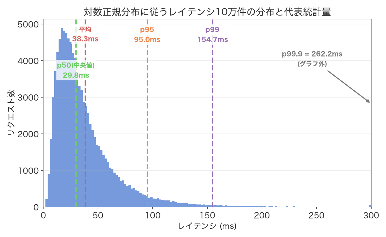
Two things stand out here. First, the mean (38.3ms) is 28% higher than the median (29.8ms). The peak of the distribution — where most requests cluster — sits near the median, and the mean is pulled to the right of it. Second, measuring directly shows that 63.9% of all requests finish faster than the mean (equivalently, 36.1% are slower). In other words, the “average request” is actually a minority experience — a single mean value does not represent the “typical” user experience.
Furthermore, p99 (154.7ms) is 5.19 times the median, and p99.9 (262.2ms) reaches 6.84 times the mean. Looking only at the average gives you no way to notice this “rare but real extreme slowness” at all. This is exactly why the average is nearly useless for measuring latency, and why percentiles are used instead.
2. Percentile Definitions and How to Read Them
A percentile is the boundary value below which a given percentage of the sorted data falls1. In the context of latency, “p99 is 200ms” means “99% of the observed requests returned within 200ms, and the remaining 1% were slower than that.”
The percentiles commonly used in practice, and how to read them:
- p50 (median): “Half the requests are faster than this, half are slower” — roughly the center of mass of the distribution. It’s pulled less by outliers than the mean, making it a better representative of the “typical” user experience.
- p95: The value that excludes only the slowest 5% — covers “everyday, somewhat-slow” requests. Commonly used for day-to-day dashboard monitoring.
- p99: Excludes only the slowest 1%. Many SLOs (Service Level Objectives) are defined at this level. It represents the “somewhat concerning slowness” that occurs roughly once per 100 requests.
- p99.9: Includes up to the slowest 0.1%. It represents the rare, worst-case slowness that occurs about once per 1,000 requests — but real, not hypothetical. Large-scale services handling thousands to tens of thousands of requests per second will hit this “rare” event many times a day, so it can’t be dismissed.
Which percentile you should watch depends on your goal, but the common principle is the same: look directly at the right side (the slow side) of the distribution, not the average. The next section covers why latency distributions tend to have this long right tail in the first place.
3. Why Latency Distributions Have Heavy Tails
The log-normal distribution used in Section 1’s experiment wasn’t chosen arbitrarily. Network and system response times are empirically known to approximate a log-normal shape2, and the intuitive reason is that latency is usually determined by a product of many factors (multiplicative variation) rather than a sum. CPU cache hit rates, lock contention, garbage collection, OS scheduling, network jitter, disk I/O, resource contention with neighboring containers — these factors act largely independently, each stretching the baseline case by some percentage. When you take the log of a product of many independent multiplicative factors, the result approaches a normal distribution (a multiplicative version of the central limit theorem), so the overall distribution ends up log-normal-like, with a long right tail3.
A heavy tail means that rare, large-outlier values keep occurring at a non-negligible rate. In a normal distribution, probability drops off rapidly the further you go from the mean; in a heavy-tailed distribution like the log-normal, values several times the mean are observed with meaningful frequency. The “p99.9 is 6.84x the mean” result from Section 1 is exactly this property showing up in practice.
Summarizing a heavy-tailed distribution with a single average lets that one number get dragged around by rare, extreme values. As an extreme illustration: if 99 users get a 1-second response and just 1 user waits 10 minutes (600 seconds), the average comes out to roughly 6.99 seconds — nearly 7 times what 99% of users actually experienced2. This is exactly why the average tends to diverge so far from the majority experience, and it’s the core reason to avoid it in latency monitoring.
4. Pitfall 1: You Can’t Average Percentiles
Once people start using percentiles, there’s a very common next mistake: “if I compute p99 on each of 10 servers, averaging those p99s should give me the overall p99.” This is statistically wrong, and Prometheus’s own documentation makes the point explicitly:
aggregating the precomputed quantiles from a summary rarely makes sense. In this particular case, averaging the quantiles yields statistically nonsensical values.4
Let’s measure exactly how far off this gets in practice. Of 10 servers, 9 follow the same reasonably well-behaved log-normal distribution, while the remaining 1 has a much heavier tail — as if it were struggling with disk I/O or GC pauses.
import numpy as np

rng = np.random.default_rng(7)
N_PER_SERVER = 50_000
N_SERVERS = 10

mu_normal, sigma_normal = np.log(20.0), 0.5   # 9 normal servers
mu_bad, sigma_bad = np.log(20.0), 1.3          # 1 skewed, heavy-tailed server

all_latencies, per_server_p99 = [], []
for i in range(N_SERVERS):
    if i == N_SERVERS - 1:
        lat = rng.lognormal(mean=mu_bad, sigma=sigma_bad, size=N_PER_SERVER)
    else:
        lat = rng.lognormal(mean=mu_normal, sigma=sigma_normal, size=N_PER_SERVER)
    all_latencies.append(lat)
    per_server_p99.append(np.percentile(lat, 99))

avg_of_p99 = np.mean(per_server_p99)
overall_p99 = np.percentile(np.concatenate(all_latencies), 99)
Measured results:
| Metric | Value |
|---|---|
| p99 of each of the 9 normal servers | 62.9–65.0ms |
| p99 of the one skewed server | 407.2ms |
| Simple average of per-server p99 | 98.4ms |
| p99 over all pooled requests (ground truth) | 108.5ms |
| Relative error | 9.3% |
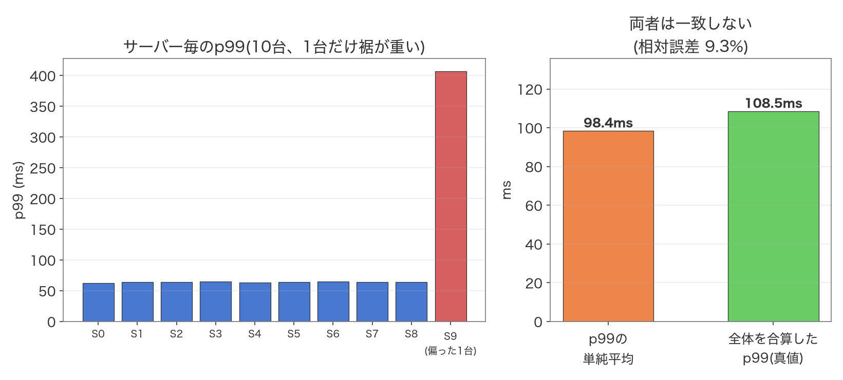
The “simple average of per-server p99” (98.4ms) and the “true p99 over all pooled requests” (108.5ms) differ by a 9.3% relative error. And this is actually a mild case — the error grows further depending on the proportion and heaviness of the skewed server’s tail. The reason is straightforward: a percentile is a non-linear statistic that depends on the entire shape of the distribution, and it doesn’t play well with a linear operation like “sum and divide.” The 99th-percentile point of the combined distribution (9 normal servers plus 1 skewed one) simply cannot be reconstructed by averaging the individual servers’ 99th-percentile points.
The correct way to combine them is not to average the already-processed percentile numbers, but to first merge the raw distributions (bucketed histogram counts), and compute the percentile exactly once on the merged result. This is precisely what Prometheus’s histogram_quantile() function does with histogram-type metrics4 — fundamentally different from a design where each instance’s summary-type metric precomputes its own percentile and those get averaged or aggregated afterward.
5. Pitfall 2: Coordinated Omission
Even if you’re computing percentiles correctly, the measurement method itself can be flawed in a way that makes results look better than reality. This problem was systematically identified by Gil Tene (Azul Systems) in his talk How NOT to Measure Latency, where he coined the term coordinated omission56.
The typical failure pattern occurs when a load-testing tool operates in a closed-loop style — sending, say, one request per second, but waiting for the previous response before sending the next, or otherwise pacing on a fixed interval tied to completion. If the system temporarily stalls and requests that should have gone out every second instead only manage to go out every 10 seconds, then all the requests that should have been sent during that 10-second stall — but weren’t — simply vanish from the measurement entirely. Those missing samples are precisely the ones that would have been sent during the period the system was stalled, so if they had actually been measured, they would have recorded very slow values. In other words, the samples that would have been the worst are the ones selectively omitted from measurement, so the measured percentiles end up looking far better than reality.
Tyler Treat’s example makes just how dramatic this effect can be very concrete7. Suppose a system processes requests that each take 1 millisecond, running at 100 req/s for 100 seconds, and then freezes completely for 100 seconds. The requests that should have arrived during the freeze all get processed in a burst the moment the freeze ends, and get recorded as if they’d just happened. If you naively measure only the processing time, you get a seemingly healthy-looking result — a 10.9ms average and a 1ms p99.99. But if you correctly measure the wait time actually experienced by users, the average comes out to 25 seconds and p99.99 to 100 seconds. The naive measurement tells you the system is fine for production — and that’s a flat-out lie7.
Practical steps to avoid coordinated omission:
- Use load-testing tools that issue requests at their scheduled time regardless of whether a response has arrived — an open-loop design (e.g.,
wrk2). A closed-loop tool that waits for a response before sending the next request will back off exactly when the system is struggling, hiding the very stall you’re trying to detect. - In application-side instrumentation, don’t just measure “time from starting processing to finishing it” — measure “time from when processing should have started to when it finished.” If you don’t count time spent waiting in a queue, you’ll miss the very phenomenon of a growing backlog.
6. Pitfall 3: Tail Latency Amplification (The Tail at Scale)
Understanding the properties of a single percentile isn’t enough once you apply it to a distributed system — there’s another trap waiting. It’s the “tail latency amplification” effect identified by Google’s Jeffrey Dean and Luiz André Barroso in their 2013 paper The Tail at Scale8.
Consider a system where a single user request fans out internally into calls to multiple backends, and the request only completes once every one of those calls has returned. If each backend call independently follows the same distribution with p99 = X milliseconds (a 1% chance of exceeding X ms), then the probability that at least one of the n calls exceeds X milliseconds is:
\[ P(\text{slowest response} > X) = 1 - (1 - 0.01)^n = 1 - 0.99^n \]As n grows, this probability rapidly approaches 1. Even something that “only happens 1% of the time per call” turns into roughly a 63% chance that someone hits it once you fan out to 100 calls.
We verify this theoretical result with Monte Carlo simulation. First, we estimate the single-backend-call p99 threshold from a 5-million-sample reference set. Then, for n = 1 through 100 parallel calls, we simulate 300,000 requests per value of n and measure “the fraction of requests where the slowest of the n calls exceeded the threshold.”
import numpy as np

rng = np.random.default_rng(2026)
mu, sigma = np.log(20.0), 0.6

# Estimate the p99 threshold from a reference sample
ref = rng.lognormal(mean=mu, sigma=sigma, size=5_000_000)
threshold_p99 = np.percentile(ref, 99)  # -> 80.876 ms

N_REQUESTS = 300_000
for n in [1, 2, 5, 10, 20, 50, 100]:
    calls = rng.lognormal(mean=mu, sigma=sigma, size=(N_REQUESTS, n))
    slowest = calls.max(axis=1)
    empirical_prob = (slowest > threshold_p99).mean()
    theory_prob = 1.0 - (0.99 ** n)
Measured results:
| Parallel calls n | Theory \(1-(0.99)^n\) | Measured | Relative error |
|---|---|---|---|
| 1 | 1.0% | 1.03% | 2.6% |
| 2 | 2.0% | 1.96% | 1.5% |
| 5 | 4.9% | 4.97% | 1.4% |
| 10 | 9.6% | 9.54% | 0.3% |
| 20 | 18.2% | 18.17% | 0.2% |
| 50 | 39.5% | 39.53% | 0.1% |
| 100 | 63.4% | 63.12% | 0.4% |
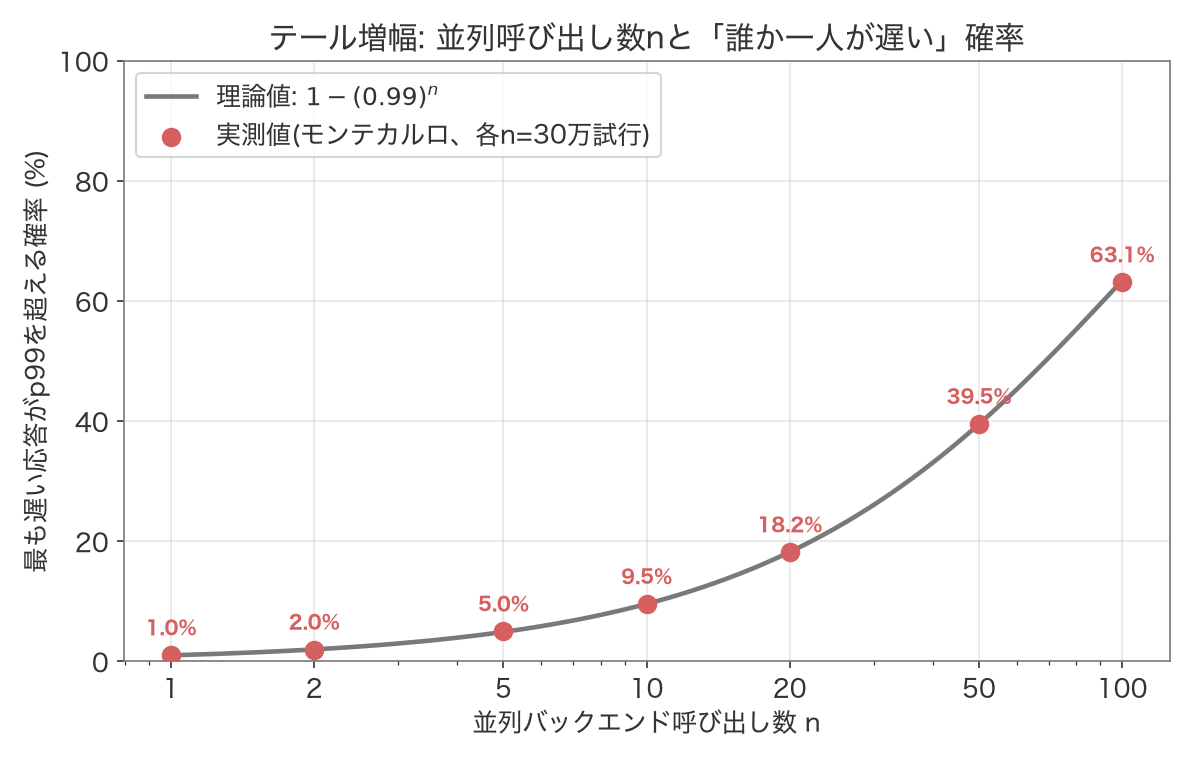
Theory and measurement agree to within 3% relative error at every value of n, confirming that the simple formula \(1-(0.99)^n\) accurately describes tail amplification behavior under the idealized assumption of independent, identically distributed (iid) calls.
This phenomenon isn’t just a theoretical concern. In the same paper, Dean & Barroso also report a real measurement from a Google production service: the 99th-percentile latency for a single request measured at the root is 10ms, but the 99th-percentile latency for all the fanned-out requests to a large number of leaf servers to finish reaches 140ms — and waiting for just the slowest 5% of those requests accounts for half of that overall 99th-percentile latency8. In a real service, individual calls aren’t perfectly iid — they’re correlated — so the exact numbers don’t match the simple iid calculation above. But the qualitative conclusion holds in both the idealized experiment and the real production measurement: the slowness of a parallelized call is amplified more severely than the slowness of any individual call.
In modern microservice architectures, where a single request can fan out into dozens of internal service calls, the latency the end user actually experiences can be far worse than any individual service’s p99, no matter how good that individual p99 looks. This is why p99 needs to be designed and monitored not just as a “per-backend metric,” but with an eye to how much the whole system amplifies it.
7. Practical Usage
Based on the experiments above, here’s how percentiles should be used in practice:
- Set SLOs (Service Level Objectives) against p99: Because the average represents only a minority experience, using it to judge SLO compliance can hide the fact that most users are actually satisfied — or conversely, that some users are having a genuinely bad time. Basing it on p99 (or p95/p99.9 depending on the situation) lets you directly guarantee that “nearly everyone stays within acceptable slowness.”
- Approximate with histogram buckets: Storing every raw request value to compute exact percentiles is expensive in memory and network cost. Prometheus’s
histogramtype instead keeps cumulative counts per predefined bucket boundary, andhistogram_quantile()linearly interpolates between buckets to approximate the percentile4. Finer bucket boundaries improve precision, but some error tied to bucket granularity always remains — worth keeping in mind. - When you need p99 across multiple instances, always merge the raw data (histograms) first, then compute the percentile exactly once: As measured in Section 4, averaging or weight-averaging already-computed per-instance p99 values does not give the correct answer. On the monitoring side, this means choosing
histogramoversummarytype metrics, or retaining raw pre-aggregation logs. - Check whether your load-testing/latency-measurement tools are causing coordinated omission: Verify you aren’t using a closed-loop load tester that waits for a response before sending the next request, and that your instrumentation counts time spent waiting in a queue. As shown in Section 5, skipping this check can make even a genuinely struggling system look fine under production-representative load.
- Bake in tail amplification for parallelized calls: In an architecture where one request fans out to many backend calls, the end-to-end latency can be far worse than any individual call’s p99 (Section 6). Don’t just track each service’s own p99 — monitor end-to-end latency separately, and consider mitigations like hedged requests (firing the same call to multiple backends and using whichever responds first) where needed.
For related measurement work in an adjacent area, see https://yuhi-sa.github.io/en/posts/20260716_db_pool_queueing/1/, which models connection pool sizing with queueing theory — it shares this article’s underlying theme of dealing with the tail of a distribution rather than its average.
8. Conclusion
Through three experiments — 100,000 log-normal latency samples, aggregating p99 across 10 servers, and tail amplification under parallel calls — we confirmed the following quantitatively:
- The mean (38.3ms) is 28% higher than the median (29.8ms), and 36.1% of all requests are slower than the mean. The average does not represent the “typical” experience.
- The simple average of per-server p99 across 10 servers (98.4ms) diverges by 9.3% from the true p99 over all pooled requests (108.5ms). Percentiles cannot be averaged.
- As the number of parallel backend calls n grows, the probability that the slowest response exceeds p99 rises sharply in line with the theoretical value \(1-(0.99)^n\) , exceeding 63% at n=100 (measured within 3% relative error of theory at every n).
Each of these is a real example of how percentiles — a fundamentally sound tool — can still lead you to the wrong conclusion if used carelessly. Look at percentiles instead of the average. Don’t naively average or combine percentiles. Question whether your measurement method itself is committing coordinated omission. And bake in the fact that parallelization amplifies the tail. Getting these four points right measurably changes the quality of latency-related decisions.
FAQ
Q1. Should I look at p50 or p95? A. It depends on the goal. If you want to know the “typical” user experience, p50 (median) is a better representative than the average. If you want to guarantee that the vast majority of users aren’t having a bad time, or you need to judge SLO compliance, you should look at the right side (slow side) of the distribution — p95 or p99. It’s also worth tracking the gap between p50 and p99 itself (5.19x in Section 1’s experiment) as a signal of how heavy the tail is.
Q2. Do I need to track p99.9? A. For a service with relatively low request volume (a few thousand requests a day), p99.9 often isn’t essential — with so few samples, the number gets statistically unstable. But for a large-scale service handling hundreds to thousands of requests per second, a “1-in-1,000” event at p99.9 still happens hundreds of times a day and can’t be dismissed as noise. Whether to extend monitoring to p99.9 or even p99.99 should depend on traffic volume and business criticality.
Q3. What does a gap between the mean and p50 (median) mean? A. If the two are close, the distribution is relatively symmetric and not heavily influenced by outliers. If the mean is noticeably higher than p50 (28% in Section 1’s experiment), the distribution has a strong right tail — extremely slow requests are pulling the mean upward. Tracking this gap itself gives you an early signal of tail degradation (worsening p99/p99.9) even from mean-level data alone.
Q4. How should percentiles across multiple servers/instances be combined?
A. You must not average or weight-average already-computed per-instance percentile values — as measured in Section 4, that can be off by 9.3% or more. The correct approach is to first merge the raw observations, or at minimum bucketed histogram counts, and compute the percentile exactly once on the merged data. In Prometheus, this means using histogram-type metrics rather than summary, and computing the quantile a single time after aggregation with histogram_quantile()4.
For a broader reading list, see 10 Must-Read Technical Books for Engineers .
References
Percentile. Wikipedia. https://en.wikipedia.org/wiki/Percentile ↩︎
Vitillo, R. Why You Should Measure Tail Latencies. https://robertovitillo.com/why-you-should-measure-tail-latencies/ ↩︎ ↩︎
Tail latency. Wikipedia. https://en.wikipedia.org/wiki/Tail_latency ↩︎
Histograms and summaries. Prometheus documentation. https://prometheus.io/docs/practices/histograms/ ↩︎ ↩︎ ↩︎ ↩︎
Tene, G. (2013). How NOT to Measure Latency. QCon London 2013 slides. https://www.slideshare.net/slideshow/how-not-to-measure-latency-london-oct-2013/27088981 ↩︎
Tene, G. How NOT to Measure Latency. YouTube. https://www.youtube.com/watch?v=lJ8ydIuPFeU ↩︎
Treat, T. (2015). Everything You Know About Latency Is Wrong. Brave New Geek. https://bravenewgeek.com/everything-you-know-about-latency-is-wrong/ ↩︎ ↩︎
Dean, J., & Barroso, L. A. (2013). The Tail at Scale. Communications of the ACM, 56(2), 74-80. https://cacm.acm.org/research/the-tail-at-scale/ (see also https://research.google/pubs/the-tail-at-scale/ ) ↩︎ ↩︎