What Is RAG? A Thorough Guide to How Retrieval-Augmented Generation Works and How to Build It, from Vector Search Fundamentals [2026 Edition]

When teams try to put generative AI to work in production, the wall they hit first is usually this: an LLM can be brilliant, yet it knows nothing about your organization’s latest information or the contents of your internal documents. LLMs have a knowledge cutoff — their knowledge stops at whatever point their training data was collected — and when asked about something they don’t know, they can confidently return a wrong answer anyway (hallucination). The most practical answer to both problems is RAG (Retrieval-Augmented Generation). In one sentence, RAG is a mechanism that searches an external knowledge source for relevant information before letting an LLM answer, and then generates the response with that information included in the prompt. Rather than relying solely on the LLM’s own parameters (parametric memory), it consults searchable external data (non-parametric memory) each time, so the system can return grounded, up-to-date answers.

The idea was first formalized in a 2020 paper by Patrick Lewis and colleagues. RAG is defined there as “models which combine pre-trained parametric and non-parametric memory for language generation” — pairing a pre-trained seq2seq model such as BART (parametric memory) with a dense vector index of Wikipedia retrieved via DPR (non-parametric memory). The paper proposes two formulations: RAG-Sequence, which conditions on the same retrieved passages throughout a single generation, and RAG-Token, which can draw on different passages for each generated token ( Lewis et al., “Retrieval-Augmented Generation for Knowledge-Intensive NLP Tasks,” NeurIPS 2020, arXiv:2005.11401 ). The idea this paper introduced — combining retrieval with generation — started out as a technique for academic open-domain QA, but as LLMs went mainstream from 2023 onward, it was repurposed as the most basic design pattern for letting enterprises have LLMs work with their own data.

This article is an introductory guide to RAG from an implementation-oriented perspective. This blog already has a deep dive into the core technology underpinning RAG — vector search and ANN (Approximate Nearest Neighbor search) — starting from first principles in ANN Fundamentals (in Japanese), with further articles covering the Milvus and OpenSearch implementations. This article serves as the “entry point” to that series: it surveys the RAG pipeline as a whole and shows how the individual component technologies fit together into one system. For the detailed algorithms and distance calculations behind vector search itself, we defer to the existing series articles where appropriate; here we focus on concerns specific to RAG — chunking, retrieval quality improvements, generation-side design, evaluation, and platform selection.

1. What Is RAG (Retrieval-Augmented Generation)?

Why RAG Is Needed

LLMs have three structural limitations. The first is the knowledge cutoff: an LLM only knows what happened up to the point its training data was collected, and cannot handle events or updated facts after that. The second is hallucination: because LLMs generate statistically plausible text, they can fluently produce content that has never been verified as fact. RAG mitigates this knowledge limitation by retrieving relevant information from an external knowledge base, and by grounding the generated content in a verifiable source, it is also considered to help suppress hallucination ( Hallucination Mitigation for Retrieval-Augmented Large Language Models: A Review, MDPI 2025 ). The third is organization-specific data: information such as contracts, meeting minutes, specifications, and support histories is inherently absent from an LLM’s training data, and repeatedly fine-tuning the model to reflect it is expensive and impractical. RAG instead keeps this data in an external index such as a vector database and retrieves it only when needed, letting you expand the LLM’s effective knowledge without retraining the model itself.

RAG in One Sentence

RAG is an architecture that, in response to a user’s question, first retrieves relevant documents from an external knowledge source, then passes those retrieval results as context in the prompt for an LLM to generate an answer from. The generation itself is left to the LLM’s own capability, while the “what does it know” part is swapped out for searchable external data — giving you three benefits simultaneously that fine-tuning alone doesn’t offer: updatability, verifiability, and scoped knowledge (we discuss the fine-tuning trade-off further in the FAQ).

2. How RAG Works: The Four-Step Pipeline

The RAG pipeline consists of two paths that run at different times. One is the ingestion pipeline, executed once ahead of time (or whenever the data is updated); the other is the query pipeline, executed every time a user issues a query. Figure 2-1 shows the overall picture.

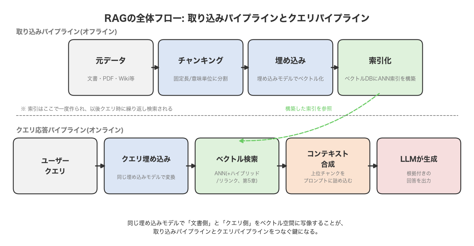
Diagram of the overall RAG flow. The top row is the ingestion pipeline, processing source data → chunking → embedding → indexing in order. The bottom row is the query pipeline, processing user query → query embedding → vector search → context assembly → LLM generates, in order. The index built by ingestion is referenced by the vector search step.

Figure 2-1: The overall RAG flow. The query pipeline (online) repeatedly searches the index built by the ingestion pipeline (offline).

The ingestion pipeline proceeds as follows. First, source data (internal documents, PDFs, wiki pages, etc.) is collected and split into manageable units through chunking. Each chunk is then converted into a fixed-length vector by an embedding model, and those vectors are indexed into a vector database. This entire preparation phase happens offline.

The query pipeline runs whenever a user actually asks a question. The user’s query is embedded with the same embedding model used at ingestion time, and a vector search (ANN) is run against the index to retrieve the most relevant chunks. Those retrieved chunks are then assembled as context in the prompt, which is passed to the LLM so it can generate a grounded answer. Mapping the “document side” and the “query side” into the same vector space using the same embedding model is the key that connects these two pipelines — and note that when you change the embedding model, the index generally needs to be rebuilt (re-embedded) as well.

The chapters that follow work through these four steps in order — chunking (Chapter 3), embedding and vector search (Chapter 4), retrieval quality improvements (Chapter 5), generation-side design (Chapter 6) — before finishing with evaluation (Chapter 7) and vector database selection (Chapter 8).

3. Chunking Strategies: Fixed-Size, Semantic, and Overlap

Chunking is the process of splitting the source document into units suited for retrieval and embedding. Embedding models have a maximum input length, and if retrieval granularity is too coarse it mixes in irrelevant information, while if it’s too fine it loses context — so how you design chunking directly affects RAG accuracy.

Fixed-Size Chunking

The simplest method is fixed-size chunking, which splits text at a fixed character or token count. In practice, chunk sizes around 200–500 tokens are common, and a starting point widely cited is to add roughly 10–20% overlap between adjacent chunks to keep sentences from being cut mid-thought ( Weaviate: Chunking Strategies for LLM Applications ). With overlap in place, even if a sentence straddles a chunk boundary, at least one of the two chunks is likely to contain the whole sentence. The weakness of naive fixed-size splitting is that it can mechanically sever information that is semantically continuous; a common mitigation is recursive chunking, which prioritizes structural boundaries such as headings and paragraphs while still respecting a maximum length.

Semantic Chunking

Semantic chunking computes sentence-level embeddings and starts a new chunk at the point where the similarity between adjacent sentence embeddings drops below a threshold (i.e., where the topic shifts). Because it splits along semantic groupings rather than character counts, it can achieve higher retrieval accuracy than fixed-size splitting on long documents that span multiple topics (such as papers or reports). On the other hand, since it requires computing an embedding for every sentence, the preprocessing cost is higher, and chunk sizes tend to become unstable depending on how the threshold is set, which is an operational challenge.

Trade-offs and Practical Guidance

Choosing a chunking strategy is always a trade-off between “preserving context” and “retrieval precision.” Larger chunks carry richer context per chunk, but are more prone to mixing in irrelevant information, which “dilutes” the embedding vector and lowers retrieval hit rate. Conversely, smaller chunks tend to raise retrieval hit rate, but a single chunk alone may not be semantically self-contained, making it easy to run into insufficient context at generation time. A common rule of thumb is that lightly-structured data like logs or conversation transcripts is well suited to fixed-size, token-based splitting, while data with clear topic shifts, such as papers or manuals, benefits from semantic chunking. In practice, the least wasteful approach is to start with a simple fixed-size-plus-overlap baseline, and switch only the parts where retrieval accuracy plateaus to semantic chunking or structure-aware splitting (respecting headings, tables, and code blocks).

4. Embeddings and Vector Search

The Role of the Embedding Model

Each chunk produced by chunking is converted into a fixed-length real-valued vector by an embedding model. Embedding models are trained so that “semantically similar sentences are mapped to nearby points in vector space” — and it’s only because of this property that “closeness in vector space” can approximate “closeness in meaning.” Dimensionality varies by model: OpenAI’s text-embedding-3-small, for example, outputs 1536-dimensional vectors, while the multilingual BAAI/bge-m3 outputs 1024-dimensional vectors ( OpenAI: New embedding models and API updates ; BGE-M3 model card, NVIDIA Build ). Higher dimensionality tends to mean greater expressive power, but index memory usage scales proportionally with it.

The semantic closeness of two vectors \(\mathbf{a}, \mathbf{b}\) is most often measured with cosine similarity:

\[ \text{sim}(\mathbf{a}, \mathbf{b}) = \frac{\mathbf{a} \cdot \mathbf{b}}{\|\mathbf{a}\| \, \|\mathbf{b}\|} \]

This metric compares only the direction of the vectors, ignoring their magnitude (norm) — a property that makes it robust to differences in text length, which is why it is a popular choice for embedding search. If the vectors are already normalized (norm of 1), cosine similarity becomes equivalent to a plain dot product, reducing computational cost.

Approximate Search via ANN

Once the number of chunks exceeds a few million, exact search (brute-force kNN) — computing the distance between the query vector and every single chunk vector — becomes computationally impractical. That’s why production systems rely on ANN (Approximate Nearest Neighbor search), which forgoes the guarantee of finding the true nearest neighbors and instead returns, with high probability, a set that’s close to them, at a small fraction of the computational cost. The mechanics of representative ANN algorithms such as HNSW, IVF, PQ, and DiskANN, why the curse of dimensionality makes approximate search necessary in the first place, and how to measure recall and QPS (queries per second) are covered down to the level of formulas and algorithms in ANN Fundamentals (in Japanese) — readers who want to go deeper should refer there. For this article, it’s enough to keep in mind the relationship that “RAG’s retrieval step is, internally, approximate nearest neighbor search via ANN.”

5. Improving Retrieval Quality: Hybrid Search, Reranking, and Query Transformation

Naive vector search alone is often not accurate enough for real-world queries. This chapter covers three representative improvement techniques — hybrid search, reranking, and query transformation. Figure 5-1 shows a typical pipeline that combines all three.

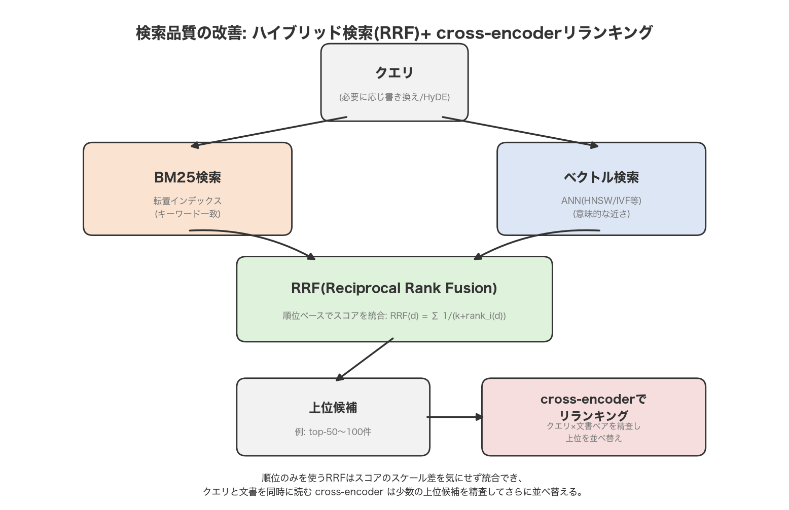
Diagram of the retrieval quality improvement flow. A query is passed to both BM25 search and vector search; their results are fused by RRF into a candidate set, which is then reranked by a cross-encoder for further reordering.

Figure 5-1: A retrieval quality improvement pipeline combining hybrid search (BM25 + vector search fused with RRF) and cross-encoder reranking.

Hybrid Search and RRF

Vector search excels at semantic closeness but is weak at “exact match on wording,” which matters for proper nouns or model numbers. Conversely, full-text search methods like BM25 excel at exact matches but are weak against vocabulary mismatch (see Chapter 1 of ANN Fundamentals (in Japanese) for details on this contrast). Hybrid search exploits this complementarity by running both kinds of search and fusing the results. A widely used fusion method is Reciprocal Rank Fusion (RRF), which uses only the “rank” — not the “raw score” — from each result list to compute a fused score for document \(d\) :

\[ \text{RRF}(d) = \sum_{i} \frac{1}{k + \text{rank}_i(d)} \]

Here \(\text{rank}_i(d)\) is the rank of \(d\) in the \(i\) -th result list, and \(k\) is a smoothing parameter, with \(k=60\) widely used empirically ( Cormack et al., “Reciprocal Rank Fusion outperforms Condorcet and Individual Rank Learning Methods,” SIGIR 2009 ; Milvus: RRF Ranker ). The practical strength of RRF is that it can fuse the results of BM25 and vector search — whose score scales are entirely different — fairly, using only rank as a common yardstick.

Reranking (Cross-Encoders)

Vector search and hybrid search embed the query and the documents separately and then compare them (the bi-encoder approach), which keeps them fast even against a large index, but this independent encoding also caps their achievable precision. A cross-encoder, by contrast, feeds a query-document pair into a single model together and outputs a score tailored to that specific combination. Because a cross-encoder requires a forward pass for every query-document pair, it can’t be applied to an entire index — so in practice, the standard approach is a two-stage architecture: use the first-stage retrieval (vector search or hybrid search) to narrow candidates down to roughly the top 50–100, and then have a cross-encoder scrutinize and reorder only those candidates ( Pinecone: Rerankers and Two-Stage Retrieval ). This extra step can substantially raise the precision of the final top-k results handed to the LLM.

Query Transformation

The query a user types can be ambiguous, too short, or phrased differently from the domain’s terminology, and using it as-is for search often hurts accuracy. To address this, it’s common to have the LLM itself rewrite the query before retrieval — a technique called query transformation. A representative method is HyDE (Hypothetical Document Embeddings): given a query, an LLM is first asked to generate a “hypothetical document” that would plausibly answer it, and that hypothetical document is embedded and used as the vector search query. The factual correctness of the generated hypothetical document isn’t the point — the method exploits the fact that its semantic pattern tends to match genuinely relevant documents ( Gao et al., “Precise Zero-Shot Dense Retrieval without Relevance Labels,” arXiv:2212.10496 ). Other common query transformation techniques include multi-query, which generates several paraphrased queries and fuses the results, and query decomposition, which breaks a complex question down into simpler sub-queries.

Practical Introduction to Vector Search (Tomohiro Manabe, Gijutsu-Hyoron-sha)

Amazonで見る

6. Generation-Side Design: Packing Context and Attaching Citations

No matter how accurate retrieval is, how you hand the retrieved chunks to the LLM has a major impact on the final answer quality.

How to Pack Context

The top-k chunks obtained from retrieval are basically listed straight into the prompt, but their order matters too. Language models handling long contexts have been reported to show a U-shaped performance curve: they perform best when relevant information sits at the very beginning or end of the input context, and their performance degrades substantially when the relevant information is buried in the middle (the so-called “lost in the middle” phenomenon; Liu et al., “Lost in the Middle: How Language Models Use Long Contexts,” TACL 2024, arXiv:2307.03172 ). Given this finding, reordering tricks — placing the most important chunks (as determined by reranking) at the start or end of the context, or ordering from least to most relevant so the single most important piece of information sits right before the query — can raise answer quality from the same retrieval results.

How to Attach Citations

One of RAG’s most practically useful properties is that it can surface the grounds for its answer. By attaching metadata such as document ID, source URL, or page number to each chunk in the prompt, and instructing the system prompt to “cite the reference number when answering,” you can get the LLM to produce footnote-style citations. This lets users trace the answer back to the primary source that grounded it, realizing RAG’s original goal of making generated content verifiable.

Living with the Context Window

A larger context window lets you pack in more chunks, but that doesn’t mean “the more, the better.” More tokens means higher inference cost and latency, and as with the lost-in-the-middle phenomenon above, mixing in irrelevant chunks can actually hurt answer quality. In practice, the two-stage design from Chapter 5 — cast a wide net at retrieval, narrow it down with reranking, and only pass the scrutinized top few chunks into the final context — is also a sensible way to make use of the context window.

7. Evaluating RAG: Retrieval Evaluation and Generation Evaluation

Evaluating RAG requires separating two distinct questions with different characteristics: “is retrieval working correctly?” and “is the generated output faithful to what was retrieved?”

Retrieval Evaluation: recall@k

For the retrieval step, the basic metric is recall@k — how much of the correct (relevant) document set is contained within the top-k retrieval results. The precise definition of recall, how to plot a recall-versus-QPS trade-off curve by sweeping a candidate-count parameter while measuring both recall and query speed (QPS) simultaneously, and cautions around benchmark design (warm-up, controlling cache state, etc.) are covered in detail in the evaluation chapter of ANN Fundamentals (in Japanese) — please refer there. In RAG specifically, it’s worth noting that if this retrieval precision is low to begin with, no amount of excellence in the downstream generation step can produce a correct answer.

Generation Evaluation: Faithfulness and Answer Relevancy

Evaluating the generation step requires different metrics than retrieval evaluation. A widely used open-source evaluation framework in this space is RAGAS (RAG Assessment), which defines four representative metrics ( Ragas: Metrics ):

Faithfulness: How faithful the generated answer is to the content of the retrieved context. A metric directly tied to hallucination detection — whether the answer includes information not present in the context.
Answer Relevancy: How precisely the generated answer addresses the user’s actual question.
Context Precision: What proportion of the retrieved context was actually relevant to generating the answer.
Context Recall: How completely the retrieved context covers the information needed to derive the correct answer.

Of these, Context Precision and Context Recall assess the quality of retrieval, while Faithfulness and Answer Relevancy assess the quality of generation, and scores are typically computed by using an LLM itself as the evaluator (LLM-as-judge). Compared to human evaluation, this is cheap to run repeatedly, but it’s worth keeping in mind that the quirks and biases of the evaluating LLM itself can leak into the scores. In practice, a realistic evaluation setup is a two-tier approach: first use recall@k to isolate whether there’s a bottleneck at the retrieval stage, then continuously monitor generation quality with Faithfulness and Answer Relevancy.

8. Choosing a Vector Database and the 2026 Trend

Two Options: Milvus and OpenSearch

When it comes to deciding where to actually place the RAG index, the two candidates that come up most often in practice are Milvus, the flagship purpose-built vector database, and OpenSearch, a full-text search engine with integrated vector search capability. Both implement the same underlying ANN algorithms internally, such as HNSW and IVF, but because Milvus was born as “a distributed system dedicated to vector search” while OpenSearch is “a full-text search engine with vector search bolted on,” they differ substantially in how they design freshness and consistency (i.e., when data becomes searchable right after being written) and in the operational skill set required. The four-axis decision framework — existing infrastructure assets, consistency requirements, filter selectivity, and the operating team’s skill set — is worked through in detail after examining each architecture in Milvus Internals (in Japanese) and OpenSearch k-NN Internals (in Japanese), and organized further in the comparison chapter of ANN Fundamentals (in Japanese). Whichever you choose as the RAG index, the final basis for the decision should be a PoC on your own data and query patterns with recall held constant, measured empirically.

The 2026 Trend: Agentic RAG

As of 2026, the discussion around RAG centers on the agentic RAG trend. Traditional RAG was a one-directional pipeline: “retrieve, then generate, done.” Agentic RAG, by contrast, dynamically switches the retrieval strategy itself based on the complexity of the question — Adaptive-RAG, which uses a classifier that judges question difficulty to choose between no retrieval, single-step retrieval, or multi-step retrieval, is a representative example ( Jeong et al., “Adaptive-RAG: Learning to Adapt Retrieval-Augmented Large Language Models through Question Complexity,” NAACL 2024, arXiv:2403.14403 ) — and increasingly adopts a configuration where an agent that judges a single retrieval as insufficient formulates a new search query on its own and repeats retrieval (multi-hop retrieval). This shift — embedding RAG not as a single “retrieve then generate” step but as a loop of “think → retrieve → rethink → retrieve again → act” — extends RAG’s applicability beyond simple FAQ answering to complex tasks that require gathering evidence spread across multiple documents.

Summary

RAG is an architecture that compensates for the structural limitations of LLMs — hallucination and knowledge cutoff — using an external, searchable knowledge source. Its mechanism can be organized into two stages: an ingestion pipeline that turns data into a searchable form through chunking and embedding, and a query pipeline that searches on the query, assembles context, and generates an answer. Because naive vector search alone rarely reaches production-grade accuracy, combining improvement techniques is the standard practice: hybrid search that merges BM25 with vector search, reranking that has a cross-encoder scrutinize a small set of top candidates, and query transformation that rewrites the query itself. Evaluation should be split between retrieval (recall@k) and generation (Faithfulness, Answer Relevancy, and so on), and finally, which platform to build all of this on should be judged against your existing assets, consistency requirements, and operational skill set. Readers who want to go deeper into the ANN principles at the heart of RAG’s vector search are encouraged to continue with ANN Fundamentals (in Japanese).

Frequently Asked Questions (FAQ)

Q. What’s the difference between RAG and fine-tuning?

Fine-tuning retrains the LLM’s own parameters on additional data — it’s well suited to teaching a model new “behavior” or “style,” but it tends to be costly and slow to keep fresh for use cases where factual knowledge changes frequently. RAG doesn’t modify the LLM itself; it only needs its external search index updated to reflect the latest information, making it well suited to data that changes often or use cases that demand verifiability. The two aren’t mutually exclusive — it’s also common in practice to fine-tune for output format or behavior while supplying factual knowledge through RAG.

Q. What kind of data is RAG suited for, and what isn’t it suited for?

Data that is searchable as text and either updated frequently or absent from the LLM’s training data — internal documents, manuals, FAQs, meeting minutes — is well suited to RAG. Conversely, tasks that require “computation or execution” rather than “retrieval,” such as simple arithmetic or strictly procedural processing, or information that exists only as undocumented tacit knowledge, cannot be handled by RAG alone.

Q. What should I check first when accuracy isn’t good enough?

The first thing to isolate is whether the problem lies in retrieval or in generation. As discussed in Chapter 7, if recall@k at the retrieval stage is low, the information needed for a correct answer never reaches the LLM in the first place, so no amount of tuning on the generation side will help. The next thing to suspect is chunking — an inappropriate chunk size or overlap easily leads to a state where information exists but isn’t retrieved, or is retrieved but has lost its context. If retrieval precision is solid but Faithfulness is low, the next move is to revisit how context is packed (Chapter 6) and the prompt’s instructions.

Q. Which vector database should I choose?

There’s no one-size-fits-all answer — the decision should be based on your existing infrastructure assets, your consistency requirements for freshly written data, the selectivity of your filtered searches, and your operating team’s skill set. If you already have OpenSearch/Elasticsearch operational assets, integration cost with OpenSearch tends to be lower; if you need to tightly control consistency right after writes, or want to push vector search performance to its limits, Milvus tends to be the stronger choice. See the detailed decision framework in ANN Fundamentals (in Japanese), and each system’s internal architecture in Milvus Internals (in Japanese) and OpenSearch k-NN Internals (in Japanese).