1. Why Rate Limiting Is Necessary
Once you expose an API or web service, you can’t avoid the design question of how many requests to allow per client. The motivations for adding rate limiting fall into three broad categories.
- Protection: A single client — malicious or not — sending a burst of requests can exhaust finite resources such as CPU, DB connections, or downstream API call budgets, degrading the experience for every other legitimate client. This can happen even without malicious intent: a buggy retry loop or a misfired batch job is enough.
- Fairness: In a multi-tenant SaaS, if one tenant runs away with resources, other tenants’ processing gets delayed — the classic “noisy neighbor” problem. Per-tenant limits guarantee a fair allocation.
- Protecting billing and contracts: For metered APIs (payments, LLM inference, etc.), rejecting requests that exceed the plan’s limit up front prevents unintended cost overruns and violations of contractual limits with downstream vendors.
The standard way to respond to a request that hits a rate limit over HTTP is the 429 Too Many Requests status code. It was defined in 2012 by
RFC 6585
, which states plainly: “The 429 status code indicates that the user has sent too many requests in a given amount of time.” RFC 6585 also recommends attaching a Retry-After header telling the client when it may retry (e.g., Retry-After: 3600 for a retry an hour later); the general specification of this header itself is defined in
RFC 9110 Section 10.2.3
. RFC 6585 also states explicitly that 429 responses must not be cached.
This article focuses on the decision logic itself — the algorithm that decides whether to return that 429 — rather than the response format. We confirm the classical definitions of the four standard approaches — fixed window counter, sliding window counter, token bucket, and leaky bucket — then hand-implement each in Python and measure how they actually respond to the same request patterns. How a client should behave after receiving a 429 is covered separately in our article on exponential backoff, https://yuhi-sa.github.io/en/posts/20260720_exponential_backoff/1/; this article stays focused on the server-side decision algorithm.
2. Fixed Window Counter
The simplest approach is the Fixed Window Counter. Time is divided into windows of a fixed width (e.g., one second or one minute), and a counter tracks the number of requests per window. Requests are allowed until the counter reaches the limit, after which everything is rejected until the window rolls over.
def fixed_window(timestamps, limit, window):
    allowed = []
    counts = {}
    for t in timestamps:
        w = int(t // window)          # which window this request falls into
        c = counts.get(w, 0)
        if c < limit:
            counts[w] = c + 1
            allowed.append(True)
        else:
            allowed.append(False)
    return allowed
The implementation only needs a mapping from “window number” to “count” per key (e.g., client ID), so memory usage per key is constant (O(1)), and it can be implemented in Redis with nothing more than INCR and EXPIRE. This simplicity is its biggest advantage, but it has a structural flaw: it is vulnerable to attacks that straddle the window boundary.
Let the window width be \(W\) and the limit be \(N\) . If an attacker sends \(N\) requests right at the end of window \(k\) (just before the boundary) and another \(N\) requests right at the start of window \(k+1\) (just after the boundary), the fixed window counter sees both windows as “count \(N\) /\(N\) , within limit.” But looking at any window of width \(W\) that straddles the boundary, the closer you get to the boundary, the more this span can contain up to \(2N\) requests. In other words, even though each window’s limit is individually respected, the effective instantaneous rate can reach up to twice the intended limit. This problem is also called out in Cloudflare’s blog post , which notes that fixed windows have the weakness that “because the counter resets periodically, spikes of legitimate traffic could be allowed through.” We measure this phenomenon with real numbers in the experiment (Pattern C) in Section 6.
3. Sliding Windows (Log and Counter Approximation)
The direction that resolves the fixed window’s boundary problem is the Sliding Window, which splits into two broad implementation strategies depending on how strict you need to be.
The sliding window log records the actual timestamp of every request as it arrives; at decision time it discards any timestamp older than “current time − window width” and compares the remaining count to the limit. This is exact, but it must retain one timestamp per request that falls within the window, so memory usage grows in proportion to traffic volume (O(N)) — a non-trivial cost in environments with high-frequency traffic and many clients, even using something like a Redis Sorted Set.
from collections import deque

def sliding_window_log(timestamps, limit, window):
    allowed = []
    log = deque()  # timestamps of allowed requests
    for t in timestamps:
        while log and log[0] <= t - window:
            log.popleft()
        if len(log) < limit:
            log.append(t)
            allowed.append(True)
        else:
            allowed.append(False)
    return allowed
In contrast, the sliding window counter keeps only two numbers: the count of the immediately preceding fixed window (count_prev) and the count of the current window (count_curr). It assumes traffic in the previous window was distributed uniformly, and linearly interpolates an estimated effective count for the current instant.
def sliding_window_counter(timestamps, limit, window):
    allowed = []
    counts = {}
    for t in timestamps:
        w = int(t // window)
        elapsed = t - w * window
        prev = counts.get(w - 1, 0)
        curr = counts.get(w, 0)
        est = prev * (1 - elapsed / window) + curr
        if est < limit:
            counts[w] = curr + 1
            allowed.append(True)
        else:
            allowed.append(False)
    return allowed
This is exactly the approach described in Cloudflare’s blog post “counting things, a lot of different things” , which cites its benefits as “small memory footprint: only two numbers per counter” and “simple to compute: one GET command plus basic arithmetic,” and notes it can be implemented using only memcache’s GET/SET/INCR. Unlike the exact log-based approach, this is an approximation — worth keeping in mind — so if traffic in the previous window was actually skewed (e.g., clustered at its tail), the estimate will drift somewhat from reality. Still, as we confirm in Section 6, in practice it’s accurate enough to substantially mitigate the fixed window’s “up to 2x” problem.
4. Token Bucket
The Token Bucket models a bucket with capacity b that is continuously refilled at a steady rate r. Every incoming request consumes one token from the bucket; if a token is available, the request is allowed, and if the bucket is empty, it is rejected. Once the bucket is full, additional tokens are simply discarded (the bucket doesn’t overflow above capacity).
- Refill rate \(r\) : determines the long-term average rate the system is willing to sustain.
- Burst capacity \(b\) : if the client has been idle long enough for the bucket to fill up, that surplus lets it push through a momentary burst above \(r\) all at once — effectively a “savings” cap.
def token_bucket(timestamps, rate, capacity):
    allowed = []
    tokens = capacity
    last = timestamps[0] if timestamps else 0.0
    for t in timestamps:
        tokens = min(capacity, tokens + (t - last) * rate)  # refill proportional to elapsed time, capped at capacity
        last = t
        if tokens >= 1.0:
            tokens -= 1.0
            allowed.append(True)
        else:
            allowed.append(False)
    return allowed, tokens
Token buckets are extremely common in practice. Stripe uses a token bucket for its own API rate limiting, explaining that it keeps the average request rate steady while still tolerating momentary traffic spikes such as flash sales (see this write-up on Stripe’s rate limiters and Stripe’s own engineering blog ). Because \(r\) and \(b\) can be tuned independently, it’s a strong fit for requirements like “keep the long-term average strict, but don’t kill short-term jitter from legitimate clients.”
5. Leaky Bucket
The Leaky Bucket is often contrasted with the token bucket, and conceptually it’s almost the inverse. Water (requests) is poured into the bucket irregularly, but a hole in the bottom of the bucket lets water leak out at a constant rate at all times (i.e., requests are processed at a fixed rate). Any amount beyond the bucket’s capacity overflows and is discarded (rejected). Where the token bucket controls “admission” itself, the leaky bucket controls the actual rate at which requests get processed, smoothing it — a fundamentally different target.
nginx’s ngx_http_limit_req_module implements exactly this “leaky bucket” method for rate limiting. Per the
official documentation
, the configuration looks like this:
limit_req_zone $binary_remote_addr zone=one:10m rate=1r/s;

server {
    location /search/ {
        limit_req zone=one burst=5;  # average 1r/s, absorb bursts up to 5 by queueing
    }
}
rate is the leak rate (the smoothed average processing rate), and burst is the maximum number of requests the queue can hold. Requests beyond burst are discarded (a 503 error by default). The nodelay option processes the burst allowance immediately instead of delaying it, though those requests are still counted against the limit.
Rather than literally simulating each request sitting in a queue with discrete events, our implementation uses a virtual queue level technique (equivalent to the well-known GCRA — Generic Cell Rate Algorithm — implementation). We track level, a virtual measure of “how much is currently queued/pending,” and let it leak away over elapsed time — reproducing identical behavior without simulating each queued request individually.
def leaky_bucket(timestamps, rate, capacity, init_level=0.0):
    allowed = []
    depart_times = []       # scheduled time each request is actually processed (departs)
    level = init_level
    last = timestamps[0] if timestamps else 0.0
    for t in timestamps:
        level = max(0.0, level - (t - last) * rate)  # leak proportional to elapsed time
        last = t
        if level < capacity:
            level += 1.0
            allowed.append(True)
            depart_times.append(t + level / rate)     # this request's scheduled completion time
        else:
            allowed.append(False)
            depart_times.append(None)
    return allowed, depart_times, level
The key implementation detail is that “admission (can it fit in the queue)” and “the actual time of processing” are decoupled — and this property shows up as a striking difference in the burst experiment in Section 6.
6. Experiment: Applying All Four Algorithms to the Same Traffic
First, let’s lay out how the four mechanisms work, visually.
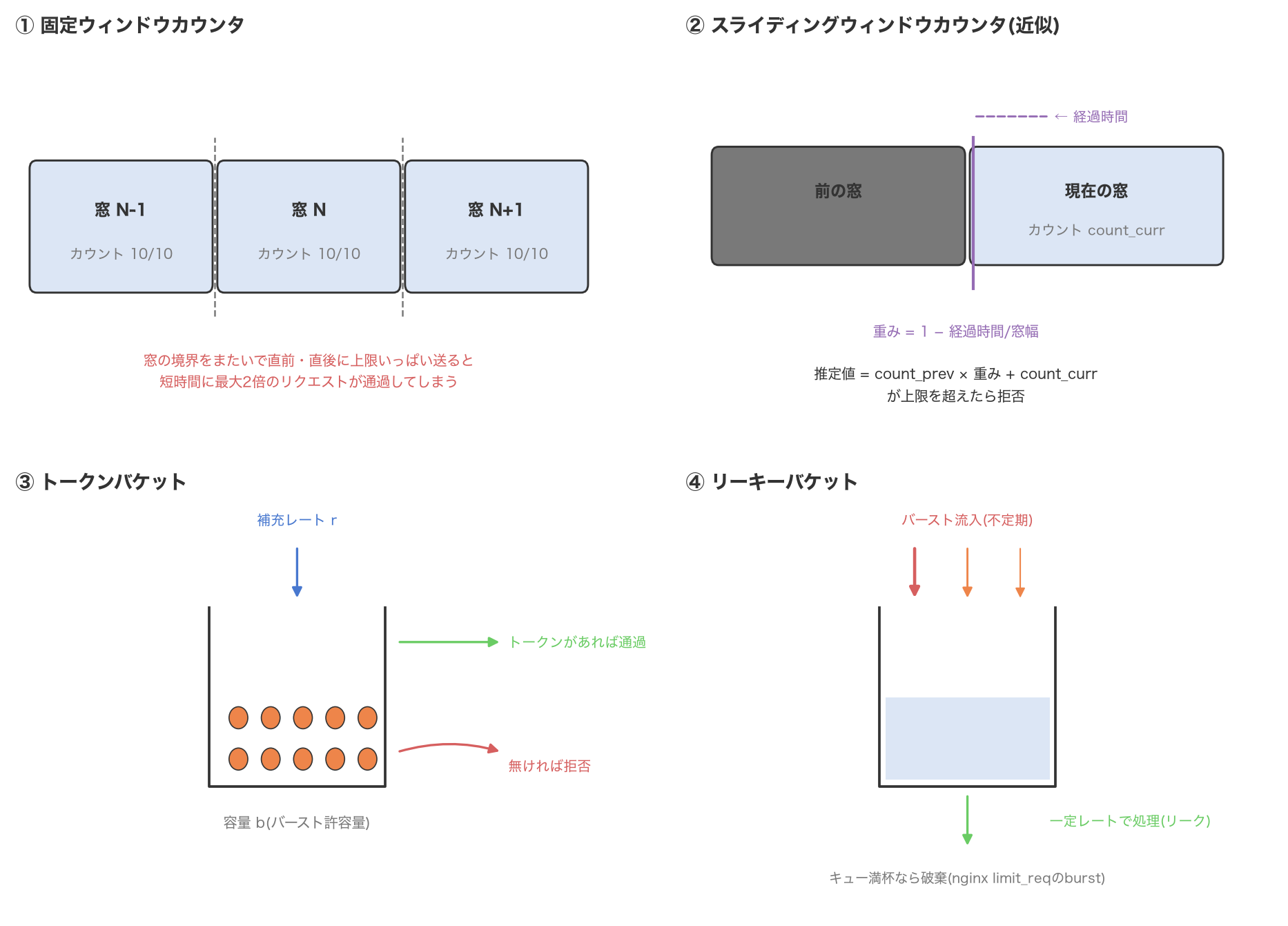
For the experiments below, we standardized on the following configuration: the two window-based methods (fixed window, sliding window counter) use limit=10 (a window width of 1 second, i.e., equivalent to 10 req/s); the token bucket uses refill rate r=10 tokens/s and capacity b=20; the leaky bucket uses processing rate rate=10 req/s and queue capacity 20. All random seeds are fixed at 42. The full experiment code is collected in rate_limit_sim.py, and every number below is an actual measurement from running that script.
Pattern A: Uniform Request Flow (Normal Operation)
First, we generate a 30-second request sequence from a Poisson process at an average rate of 6 req/s (60% of the 10 req/s limit) using random.Random(42).expovariate(6.0), and feed it into all four algorithms simultaneously. The generated sequence contained 184 requests in total.
| Algorithm | Allowed | Rejected | Allow rate |
|---|---|---|---|
| Fixed window | 178 | 6 | 96.74% |
| Sliding window counter | 178 | 6 | 96.74% |
| Token bucket (b=20) | 184 | 0 | 100.00% |
| Leaky bucket (capacity 20) | 184 | 0 | 100.00% |
Even with an average rate at only 60% of the limit, a Poisson process produces chance clustering (moments where arrivals happen to bunch up), so the two window-based methods hit their cap for that instant and rejected 6 requests. Token bucket and leaky bucket, on the other hand, have enough buffer (b=20 / capacity 20) to absorb normal-operation jitter, so they allowed every request. It’s also notable that the fixed window and sliding window counter allowed the exact same number (178) — when count_prev is near zero, as it is under normal conditions, the two behave nearly identically, which we can confirm directly from the measurement. Under normal-operation traffic, all four algorithms behave “roughly equivalently,” as expected.
Pattern B: Burst (Instantaneous Concentration)
Next, we ran a pattern with 5 seconds of idle time (the token bucket sits full at b=20, the leaky bucket’s queue is empty), followed by 30 requests fired within 20 milliseconds, followed by idle time again.
| Algorithm | Allowed | Rejected | Allow rate |
|---|---|---|---|
| Fixed window | 10 | 20 | 33.33% |
| Sliding window counter | 10 | 20 | 33.33% |
| Token bucket (b=20) | 20 | 10 | 66.67% |
| Leaky bucket (capacity 20) | 21 | 9 | 70.00% |
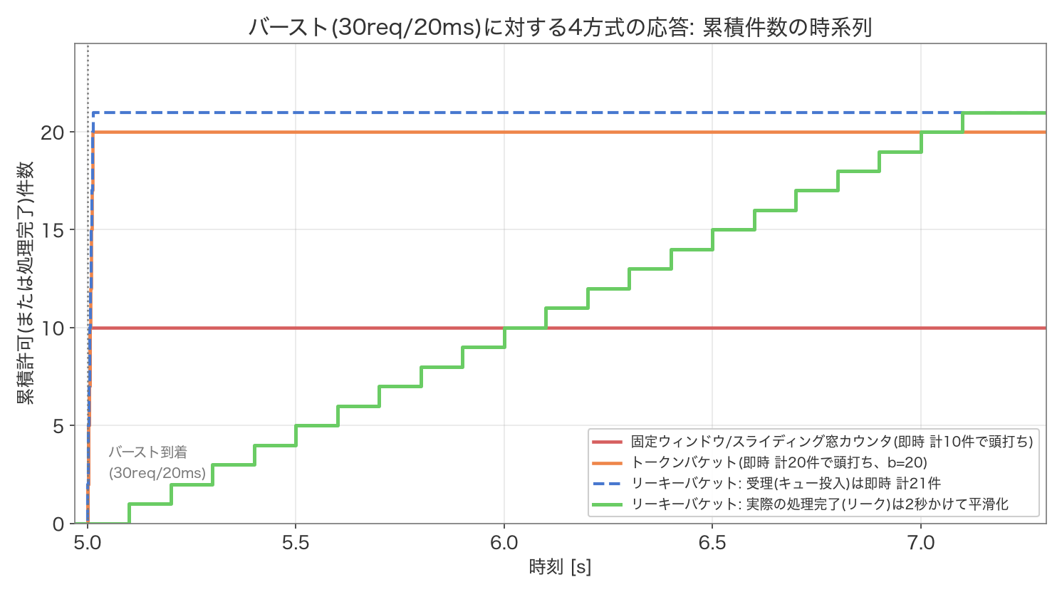
The two window-based methods hit their mechanical ceiling of 10, the window’s limit. The token bucket burns through its b=20 accumulated tokens, letting 20 requests through instantly before running dry and rejecting the rest. The leaky bucket admitted a slightly larger 21 requests into its capacity-20 queue, due to ongoing leakage during the burst itself — but the important part is when those 21 admitted requests actually get processed. Although the first and last admissions were only 20 milliseconds apart, the measured completion times were spread across 2.000 seconds, from 5.100s to 7.100s. This is consistent with the arithmetic of a leak rate of 10 req/s needing a bit over 2 seconds to work through 21 requests, and it quantitatively confirms the leaky bucket’s defining property: admission is instant, but output is smoothed to a constant rate. Where the token bucket lets an entire burst through up to its allowance, the leaky bucket accepts the burst but drains it out gradually — a qualitative difference this experiment makes vividly clear.
Pattern C: Window Boundary Attack
Finally, we measure the fixed window’s boundary problem described in Section 2. We ran three windows (0–2 seconds) of steady-state traffic at exactly the limit (10 req/window, evenly spaced), followed by window 3 ([3, 4) seconds), in which the 10 requests that would normally be evenly spaced are instead all concentrated in the last 100 milliseconds (3.90–3.99s), followed by window 4 ([4, 5) seconds), in which its 10 requests are likewise concentrated in the first 100 milliseconds (4.00–4.09s). This is the textbook scenario of “an attacker deliberately concentrates requests right before and right after a window boundary.” Token bucket and leaky bucket are subjected to the same concentrated burst, under the premise that they too had been operating under the same steady-state traffic beforehand (i.e., roughly balanced between refill/leak and consumption, with no artificial slack built up).
Here is how many requests were allowed within the 190-millisecond span straddling the boundary (3.90s–4.10s, 20 attack requests total):
| Algorithm | Allowed within the 190ms attack window |
|---|---|
| Fixed window | 20 / 20 |
| Sliding window counter | 11 / 20 |
| Token bucket | 12 / 20 |
| Leaky bucket | 20 / 20 |
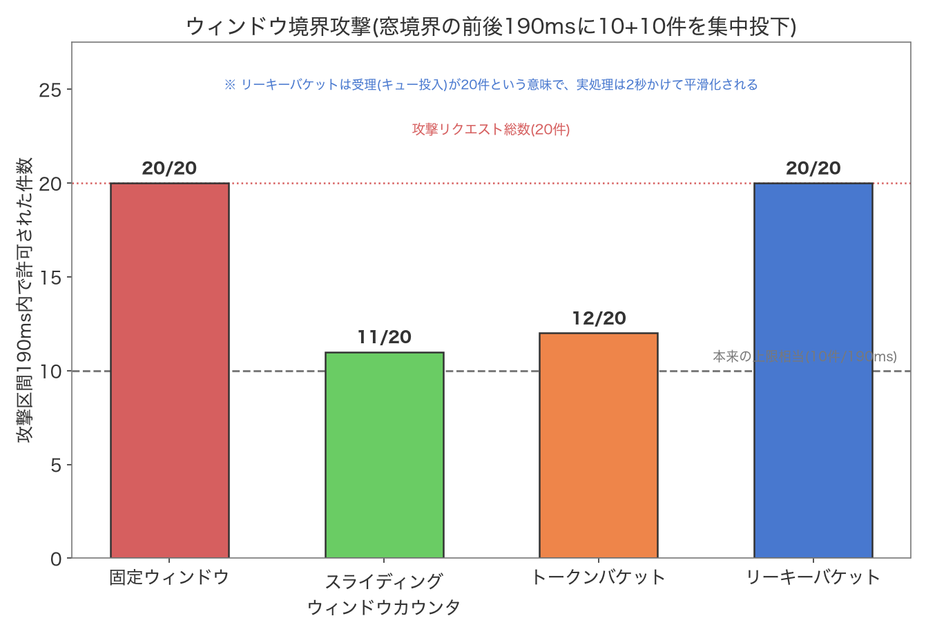
Looking at the fixed window per-window: window 3 shows 10/10 and window 4 shows 10/10 — each window individually looks “within limit.” But across the 190-millisecond span straddling the boundary, 20 requests got through in total — exactly the “up to 2x” problem from Section 2, now confirmed with a measurement that matches the theoretical prediction precisely. The sliding window counter, by contrast, still carries a heavy weight from window 3’s result (count_prev=10) by the time window 4 begins, so its estimated count is already pinned near the limit and it rejects most of window 4’s requests (9 of 10), keeping the total for the attack window down to 11/20. The token bucket is held down to 12/20 for a similar reason: having been running under steady-state traffic right up to the attack, it has no surplus of banked tokens. The leaky bucket has no concept of a “window” at all, so it admits all 20 requests — but just as in Pattern B, actual processing is smoothed out over roughly 2 seconds, so the downstream system never actually experiences an instantaneous load of 20 req/190ms. The vulnerability tied to the notion of a “window” simply does not exist, in principle, for the continuous-time token bucket and leaky bucket, and even among the window-based methods, the sliding window counter is measurably more resistant to this attack than the fixed window — a conclusion now backed by real numbers.
7. Rate Limiting in Distributed Environments
Everything so far assumed a counter held in a single process’s memory, but real services typically run multiple application servers behind a load balancer. If each server keeps its own independent in-memory counter, once a single client’s requests get spread across servers, the effective limit loosens by roughly a factor of the number of servers. The Redis rate limiter documentation makes this explicit: “Local per-process counters break behind load balancers: the same client bypasses limits by hitting different instances,” and it argues you need a centralized store shared across all instances. Redis is widely used for this, for three reasons:
- Sub-millisecond latency: checking the limit on the synchronous request path doesn’t introduce perceptible delay.
- Atomic operations: combining
INCRandEXPIREcan implement a fixed window counter, but a race condition can occur if another process’s read slips in between the two commands, leaving the TTL never set and the counter leaking forever. The standard fix is to bundle the whole sequence into a single Lua script executed withEVAL— callEXPIREonly whenINCR’s return value is 1 (i.e., this is the first request for that key). Redis’s official documentation explains that “Lua scripting with EVAL keeps the read-decide-update cycle atomic, so concurrent requests cannot double-spend tokens or lose counter updates.” Implementing a token bucket in Redis follows the same pattern: store “token count” and “last refill time” in a hash, and fold the refill calculation from elapsed time, the cap at capacity, and the consumption check all into a single Lua script — keeping network round trips to one while guaranteeing atomicity. - Automatic cleanup via TTL: fixed-window keys become unnecessary once the window has passed, and
EXPIREclears them automatically without any explicit cleanup process.
There’s also a subtlety around error introduced across multiple nodes. If every node queries a single Redis instance (or a single shard of a cluster), the decision itself is exact — but the network round-trip latency between the application server and Redis means that, under an extremely high level of concurrency, a burst can momentarily push slightly more requests through than the limit (there’s a small lag between the check and the update). And in a multi-region deployment where each region runs its own independent Redis (to avoid synchronization cost), the counters are inherently separate, so the global total ends up looser than the intended limit. The Redis documentation addresses this trade-off by describing Active-Active replication with CRDT-based eventual consistency. Facing a similar challenge at a much larger scale, Cloudflare’s engineering blog describes an edge-based rate limiter operating across millions of domains that, rather than synchronously updating a single global counter on every request, combines local approximate counting with asynchronous aggregation to minimize latency impact while still achieving sufficient accuracy. In distributed environments, “perfectly exact counting” and “low latency” are fundamentally in tension, and how much approximation to tolerate is a design decision that depends on the requirements at hand.
8. A Selection Guide
Based on the experimental results, here’s how to think about which algorithm fits which requirement.
| Requirement | Fixed window | Sliding window counter | Token bucket | Leaky bucket |
|---|---|---|---|---|
| Burst tolerance | Only within a window; weak at boundaries | Within a window; comparatively resistant at boundaries too | Explicitly tunable via b | Tolerated, but smoothed — no instantaneous throughput |
| Output smoothing | None | None | None (a burst passes through instantaneously) | Yes (structurally constant-rate) |
| Resistance to boundary attacks | Weak (measured up to 2x pass-through) | Strong (measured 11/20 suppression) | Strong (continuous-time based) | Strong (no concept of a window at all) |
| Implementation simplicity | Simplest, by far | Good (log variant is heavier, larger memory) | Good | Good (queue implementation is somewhat more involved) |
| Memory usage | O(1) | Log variant O(N); counter approximation O(1) | O(1) | O(queue length) |
| Representative use cases | Simple API thresholds, internal tools | Rate limiting at Cloudflare’s edge | Stripe’s API, burst tokens on cloud APIs | nginx limit_req, queueing to protect downstream systems |
It’s practical to work backward from what you’re actually trying to protect. If you want to smooth out load on a downstream system, choose the leaky bucket. If you want to keep the average rate strict without killing normal jitter, choose the token bucket. If you want implementation simplicity above all and can tolerate the boundary-attack risk, the fixed window is fine. If you want fixed-window-level lightness but with the boundary problem mitigated, reach for the sliding window counter.
Conclusion
We hand-implemented the fixed window counter, sliding window counter, token bucket, and leaky bucket, and ran an experiment applying all four to the same request sequences. Under normal operation (Pattern A), all four behaved roughly equivalently. Under a burst (Pattern B), we measured a clear qualitative difference: the token bucket lets a burst through instantly up to its allowance, while the leaky bucket admits it but smooths the actual processing. Under a boundary attack (Pattern C), the fixed window let through what amounts to twice the intended limit (20/20) even though each individual window looked compliant, while the sliding window counter suppressed this down to 11/20. Being able to confirm, with actual numbers from actually running the code, flaws and properties that are usually just “said” to be true theoretically was the biggest payoff of this exercise.
FAQ
Q1. What’s the difference between token bucket and leaky bucket?
Both control the average rate, but they control different things. The token bucket controls “admission” itself, and up to the burst allowance b it will let multiple requests through instantly, all at once. The leaky bucket smooths “actual processing (output)” to a constant rate. In our Pattern B experiment, the token bucket instantly allowed 20 of a 30-request burst before hitting its ceiling, while the leaky bucket admitted 21 but smoothed the actual processing out over 2 seconds — a difference we confirmed quantitatively.
Q2. What should a client do when it hits a rate limit?
Don’t retry immediately after receiving a 429 — follow the Retry-After header if present, or use exponential backoff combined with jitter to progressively widen the retry interval. We cover the concrete implementation and measurements in https://yuhi-sa.github.io/en/posts/20260720_exponential_backoff/1/.
Q3. Why is the fixed window considered bad?
It’s the simplest to implement, and it’s not a real problem under normal traffic. But as measured in Section 6, Pattern C, an attack targeting the window boundary — concentrating requests right before and right after it — can let through 20 requests within a 190-millisecond span, twice the nominal limit of 10 (fixed window 20/20 vs. sliding window counter 11/20). If you can’t tolerate that risk, choose at least the sliding window counter.
Q4. How should you decide the rate values (r, b, window size, etc.)?
Start from the measured capacity of whatever you’re actually protecting — your own server’s spare CPU, a downstream database’s processing capacity, a contractual limit with an external API, and so on. Set the refill rate r (or the fixed window’s limit) to the throughput you can sustain continuously, and, for a token bucket, add a burst allowance b large enough to absorb normal traffic jitter. A setting that’s too strict rejects legitimate users, and one that’s too lax provides no real protection, so in practice it pays to feed real traffic patterns through all four algorithms, as we did in Pattern A, and tune based on the observed rejection rate.
Related Articles
- Modeling Database Connection Pool Sizing with Queueing Theory (M/M/c) — that article is about capacity design, “how many concurrent requests can you afford to handle,” which complements this article’s focus on rate, “how many requests per unit time should you accept.”
- PID Control for HPA — an approach that dynamically adjusts the amount of resources itself in response to load; where rate limiting is a static defense that “rejects at the door,” this is a dynamic response that “increases supply, even if belatedly.”
For recommendations in other areas, see our roundup of 10 Must-Read Technical Books for Engineers .